PyLiq1 Material
- Command_Manual
- Tcl Commands
- Modeling_Commands
- model
- uniaxialMaterial
- ndMaterial
- frictionModel
- section
- geometricTransf
- element
- node
- sp commands
- mp commands
- timeSeries
- pattern
- mass
- block commands
- region
- rayleigh
- Analysis Commands
- Output Commands
- Misc Commands
- DataBase Commands
This command constructs a uniaxial p-y material that incorporates liquefaction effects. This p y material is used with a zeroLength element to connect a pile (beam-column element) to a 2 D plane-strain FE mesh or displacement boundary condition. The p-y material obtains the average mean effective stress (which decreases with increasing excess pore pressure) either from two specified soil elements, or from a time series. Currently, the implementation requires that the specified soil elements consist of FluidSolidPorousMaterials in FourNodeQuad elements, or PressureDependMultiYield or PressureDependMultiYield02 materials in FourNodeQuadUP or NineFourQuadUP elements. There are two possible forms:
| uniaxialMaterial PyLiq1 $matTag $soilType $pult $Y50 $Cd $c $pRes $ele1 $ele2 |
OR
| uniaxialMaterial PyLiq1 $matTag $soilType $pult $Y50 $Cd $c $pRes -timeSeries $tag |
| $matTag | integer tag identifying material |
| $soilType | soilType = 1 Backbone of p-y curve approximates Matlock (1970) soft clay relation.
soilType = 2 Backbone of p-y curve approximates API (1993) sand relation. |
| $pult | Ultimate capacity of the p-y material. Note that "p" or "pult" are distributed loads [force per length of pile] in common design equations, but are both loads for this uniaxialMaterial [i.e., distributed load times the tributary length of the pile]. |
| $Y50 | Displacement at which 50% of pult is mobilized in monotonic loading. |
| $Cd | Variable that sets the drag resistance within a fully-mobilized gap as Cd*pult. |
| $c | The viscous damping term (dashpot) on the far-field (elastic) component of the displacement rate (velocity). (optional Default = 0.0). Nonzero c values are used to represent radiation damping effects |
| $pRes | sets the minimum (or residual) peak resistance that the material retains as the adjacent solid soil elements liquefy |
| $ele1 $ele2 | are the eleTag (element numbers) for the two solid elements from which PyLiq1 will obtain mean effective stresses and excess pore pressures |
| $seriesTag | Alternatively, mean effective stress can be supplied by a time series by specifying the text string -timeSeries and the tag of the seriesm $seriesTag. |
NOTES:
To model the effects of liquefaction with PyLiq1, it is necessary to use the material stage updating command:
updateMaterialStage –material matNum –stage sNum
where the argument matNum is the material number (for PyLiq1) and the argument sNum is the desired stage (valid values are 0 & 1). With sNum=0, the PyLiq1 behavior will be independent of any pore pressure in the specified solidElem’s. When updateMaterialStage first sets sNum=1, PyLiq1 will obtain the average mean effective stress in the two solidElem’s and treat it as the initial consolidation stress prior to undrained loading. Thereafter, the behavior of PyLiq1 will depend on the mean effective stresses (and hence excess pore pressures) in the solidElem’s. The default value of sNum is 0 (i.e., sNum=0 if updateMaterialStage is not called). Note that the updateMaterialStage command is used with some soil material models, and that sNum=0 generally corresponds to the application of gravity loads (e.g., elastic behavior with no excess pore pressure development) and sNum=1 generally corresponds to undrained loading (e.g., plastic behavior with excess pore pressure development).
The analysis for gravity loading cannot use the "algorithm Linear" command because the relevant soil materials do not currently work properly with this command. Instead, the "algorithm Newton" or some other option must be used.
EQUATIONS and EXAMPLE RESPONSES:
The PyLiq1 material inherits the PySimple1 material, and behaves identically to the PySimple1 material if there is no excess pore water pressure (i.e., sNum = 0). The constitutive equations for the PySimple1 material are given in separate documentation and not repeated here.
The PyLiq1 material modifies the p-y behavior in response to the average mean effective stress (p′), as affected by the excess pore water pressures, in two specified solid soil elements. The PyLiq1 material is used within a zeroLength element, and that zeroLength element generally shares a node with some solid soil elements (e.g., most commonly 1, 2, or 4 solid elements in a 2D mesh). Specifying two solid soil elements allows the PyLiq1 material to depend on pore pressures above and below its nodal position (essentially covering its full tributary length). The mean effective stress is affected by changes in mean total stress and excess pore pressure. For modeling purposes, an excess pore water pressure ratio is calculated as ru = 1-p′/pc′, where pc′= mean effective consolidation stress prior to undrained loading. The average value of ru is obtained from the specified solid soil elements and used within PyLiq1. The constitutive response of PyLiq1 is then taken as the constitutive response of PySimple1 scaled in proportion to the mean effective stress within the specified solid soil elements. This means that the ultimate capacity (pult) and tangent modulus are scaled by a factor of (1-ru). Two additional constraints are then placed on the constitutive response. The first is that the scaled ultimate capacity cannot fall below the specified residual capacity of the material (i.e., pRes). The second constraint applies to the situation where the mean effective stress in the adjacent solid soil elements is incrementally increasing [e.g., the pore pressures decrease as the soils are incrementally dilatant (phase transformation)]. In this “hardening” situation, the loading path from the p-y relation at time “i” to time “i+1” is bounded by the material’ elastic stiffness (i.e., the unload/reloading stiffness); e.g., the incremental loading path cannot be steeper than the elastic stiffness. Note that the above approach only provides a first-order approximation for the softening effects of liquefaction on p y behavior.
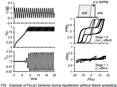
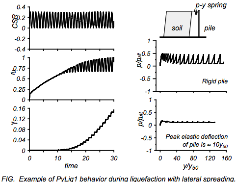
Two simple examples of PyLiq1 behavior are presented in the following figures. In these examples, there is a single FourNodeQuad element containing a FluidSolidPorousMaterial with a PressureDependMultiYield soil material. This solid element is connected to an elastic pile via a single “p-y” element (i.e., a zeroLength element containing a PyLiq1 material). The solid element is an order of magnitude stiffer than the p-y element, and is subjected to transient cyclic simple shear loading.
In the first example (first Figure), the adjacent soil element is subjected to uniform cyclic loading that produces triggering of liquefaction (ru = 100%) in about 7 cycles. The cyclic shear stress ratio (CSR), excess pore water pressure ratio (ru), and shear strain (γ) versus cycle number for the solid soil element are plotted on the left side of the Figure. The soil element experiences uniform cyclic deformations; e.g., lateral spreading does not develop because the horizontal cyclic loading has no static bias in either direction. The pile is set as relatively rigid. Two different cases are then presented for the p-y element response. In the first case, sNum=0 such that the p-y element is independent of changes in mean effective stress (or excess pore pressure) in the soil element. The resulting behavior is shown in the upper right-hand plot of the Figure. In the second case, sNum was set to 1 prior to cyclic loading, and thus the resulting behavior is dependent on the excess pore pressure in the soil element (lower right-hand plot of the Figure). The p-y element exhibits the overall softening that is expected when the adjacent soil element liquefies, and also shows temporary stiffening (hardening) when the adjacent soil goes through phase transformation (with its associated drop in excess pore pressure). In these plots, the “p” is normalized by the pult for drained monotonic loading.
In the second example (second Figure), the adjacent soil element is subjected to a static shear load plus uniform cyclic loading such that triggering of liquefaction is accompanied by progressive lateral deformation in the direction of the static load bias (i.e., lateral spreading). Again, the left side of the Figure shows the CSR, ru and γ versus cycle number for the solid soil element. sNum was set to 1 prior to cyclic loading such that the p-y behavior is dependent on the excess pore pressure in the soil element. The residual capacity (pRes) of the p-y material is 10% of the drained ultimate capacity. Two different cases are then presented. In the first case, the pile is set as relatively rigid. The resulting behavior is shown in the upper right-hand plot of the Figure. The peak “p” occurs just as triggering of liquefaction occurs in the soil element, and is about 0.49 times the drained monotonic capacity pult. Subsequent peaks in “p” drop a bit to about 0.46 times pult. In the second case, the pile has a finite elastic stiffness such that it’s peak elastic deflection in this example is equal in magnitude to about 10 times the y50 value for the p-y element. The resulting behavior is shown in the lower right-hand plot of the Figure. Again, the peak “p” occurs just as triggering of liquefaction occurs in the soil element, being about 0.18pult in this case. Subsequent peaks in “p” drop by about 20% to about 0.14pult. The inclusion of pile flexibility reduced, by a factor of about 3, the peak values of “p” that developed in the p-y element as the soil progressively spread past the pile. During each cycle of loading, the soil element cyclically ratchets in the direction of the static load bias and alternates between being extremely soft (ru = 100%) and then stiffening when it goes through phase transformation (ru drops). As the soil stiffens, the p-y element gains strength, transferring load onto the pile and causing the pile to elastically deform in the direction of loading. Then when the soil is unloaded and ru becomes 100% again, the p-y element loses strength, unloading the pile and allowing the pile to elastically return closer to its undeformed position. In each cycle of loading and progressive spreading of the soil, the magnitude of “p” that develops against the pile depends on the pile’s flexibility relative to the displacement range over which the soil goes through phase transformation.
EXAMPLE:
model basic -ndm 2 -ndf 2
node 1 0.0 0.0
node 2 0.0 0.0
fix 2 1 1
fix 1 0 1

timeSeries Path 1 -fileTime time.txt -filePath meanStress.txt -factor -1.0
uniaxialMaterial PyLiq1 1 2 1.0 0.0001 10.0 0.0 0.10 -timeSeries 1
element zeroLength 1 1 2 -mat 1 -dir 1
uniaxialMaterial TzLiq1 2 1 1.0 0.0001 0.0 -timeSeries 1
element zeroLength 2 1 2 -mat 2 -dir 1
updateMaterialStage -material 1 -stage 1
updateMaterialStage -material 2 -stage 1

recorder Element -file PY1.txt -time -ele 1 force
recorder Element -file TZ1.txt -time -ele 2 force
recorder Node -file NodalDisps1.txt -time -node 1 -dof 1 2 disp

pattern Plain 1 "Sine 0.0 10.0 1.0 -factor 1.0" {
    sp 1 1 0.001
}

system ProfileSPD
test NormDispIncr 1.0E-8 25 0
constraints Penalty 1.e18 1.e18
algorithm Newton
numberer RCM
integrator Newmark 0.6 0.30
analysis VariableTransient
analyze 1000 0.01 0.0001 0.01 15
REFERENCES:
"Seismic Soil-pile-strcture interaction experiments and analysis", Boulanger, R.w., Curras, C.J., Kutter, B.L., Wilson, D.W., and Abghari, A. (1990). Journal of Geotechnical and Geoenvironmental Engineering, ASCS, 125(9):750-759.
Code Developed by: Ross Boulanger, UC Davis This command is used to construct a PySimple1 uniaxial material object:

