UVCuniaxial (Updated Voce-Chaboche)
- Command_Manual
- Tcl Commands
- Modeling_Commands
- model
- uniaxialMaterial
- ndMaterial
- frictionModel
- section
- geometricTransf
- element
- node
- sp commands
- mp commands
- timeSeries
- pattern
- mass
- block commands
- region
- rayleigh
- Analysis Commands
- Output Commands
- Misc Commands
- DataBase Commands
This command is used to construct an Updated Voce-Chaboche (UVC) material for uniaxial stress states. This material is a refined version of the classic nonlinear isotropic/kinematic hardening material model based on the Voce isotropic hardening law and the Chaboche kinematic hardening law. The UVC model contains an updated isotropic hardening law, with parameter constraints, to simulate the permanent decrease in yield stress with initial plastic loading associated with the discontinuous yielding phenomenon in mild steels. Details regarding the model, and implementation, can be found in the cited references at the end.
| uniaxialMaterial UVCuniaxial $matTag $E $fy $QInf $b $DInf $a $N $C1 $gamma1 <$C2 $gamma2 $C3 $gamma3 … $C8 $gamma8> |
| $matTag | Integer tag identifying the material. |
| $E | Elastic modulus of the steel material. |
| $fy | Initial yield stress of the steel material. |
| $QInf | Maximum increase in yield stress due to cyclic hardening (isotropic hardening). |
| $b | Isotropic hardening saturation rate, b > 0. |
| $DInf | Difference between initial and steady-state yield stresses, to neglect the model updates set DInf = 0. |
| $a | Saturation rate of yield stress difference, a > 0. If DInf == 0, then a is arbitrary (but still a > 0). |
| $N | Number of backstresses to define, N >= 1. |
| $C1 | Kinematic hardening parameter associated with backstress component 1. |
| $gamma1 | Saturation rate of kinematic hardening associated with backstress component 1. |
| <$C2 $gamma2 $C3 $gamma3 … $C8 $gamma8> | Additional backstress parameters, up to 8 may be specified. If C is specified, then the corresponding gamma must also be specified. Note that only the first N backstresses will be read by the parser. |
Examples
1. Validation:
This first example compares the response of the UVC model with the built-in nonlinear isotropic/kinematic material model in Abaqus. For this validation the model updates are neglected by simply setting DInf = 0.0 and a = 1.0. The model parameters are:
E = 179800 MPa, fy = 318.5 MPa, QInf = 100.7 MPa, b = 8.0, DInf = 0.0 MPa, a = 1.0, C1 = 11608.2 MPa, gamma1 = 145.2, C2 = 1026.3 MPa, gamma2 = 4.7
Figure 1 shows that the two implementations agree to the level of machine precision. The finite element models used to generate the Abaqus and OpenSees responses can be found at https://github.com/ahartloper/UVC_MatMod.

2. Structural steels:
Accuracy of the UVC material model for structural steels is demonstrated through two comparisons with experimental data from uniaxial coupon tests. A comparison with a North American steel, A992 Gr. 50 (nominal fy = 345 MPa), is shown in Figure 2. A comparison with a European steel, S355J2+N (nominal fy = 355 MPa), is shown in Figure 3. In both cases the UVC model is able to represent well the initial yield stress as well as the material behavior in later loading cycles.
The parameters used in both these examples are provided in the next section.
-
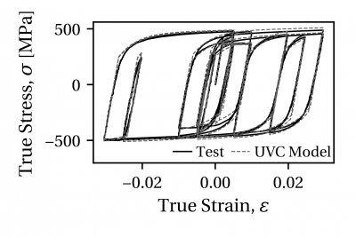
Figure 2. Comparison of UVC model with uniaxial coupon test data from the A992 Gr. 50 W14X82 flange data set.
-
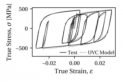
Figure 3. Comparison of UVC model with uniaxial coupon test data from the S355J2+N 25 mm plate data set.


Parameters for structural steels
Below is a list of model parameters for 12 structural steels from reference [2]. This reference also contains detailed information on the calibration procedure used to obtain the model parameters. The UVC model calibration procedure is implemented in the open-source Python package RESSPyLab, and can be used to generate parameters for applicable materials.
| UVC Material Parameters | ||||||||||
|---|---|---|---|---|---|---|---|---|---|---|
| Material | E | fy | QInf | b | DInf | a | C1 | gamma1 | C2 | gamma2 |
| - | [GPa] | [MPa] | [MPa] | - | [MPa] | - | [MPa] | - | [MPa] | - |
| S355J2+N (50 mm plate) | 197.31 | 338.80 | 134.32 | 14.71 | 133.75 | 229.25 | 26242.00 | 199.04 | 2445.30 | 11.66 |
| S355J2+N (25 mm plate) | 185.97 | 332.18 | 120.48 | 8.14 | 93.15 | 261.75 | 21102.00 | 173.60 | 2300.60 | 10.42 |
| S460NL (25 mm plate) | 187.61 | 439.20 | 97.35 | 14.02 | 136.64 | 226.40 | 26691.00 | 188.75 | 2892.40 | 10.44 |
| S690QL (25 mm plate) | 188.63 | 685.39 | 0.11 | 0.11 | 132.30 | 285.15 | 34575.00 | 185.16 | 3154.20 | 20.14 |
| A992 Gr. 50 (W14X82 web) | 210.74 | 378.83 | 122.63 | 19.74 | 143.49 | 248.14 | 31638.00 | 277.32 | 1548.60 | 9.04 |
| A992 Gr. 50 (W14X82 flange) | 191.02 | 373.72 | 141.47 | 15.20 | 135.95 | 211.16 | 25621.00 | 235.12 | 942.18 | 3.16 |
| A500 Gr. B (HSS305X16) | 191.21 | 324.09 | 228.02 | 0.11 | 50.41 | 270.40 | 17707.00 | 207.18 | 1526.20 | 6.22 |
| BCP325 (22 mm plate) | 178.61 | 368.03 | 112.25 | 10.78 | 105.95 | 221.92 | 20104.00 | 200.43 | 2203.00 | 11.76 |
| BCR295 (HSS350X22) | 178.74 | 412.21 | 0.09 | 0.09 | 103.30 | 212.83 | 20750.59 | 225.26 | 1245.04 | 2.09 |
| HYP400 (27mm plate) | 189.36 | 454.46 | 62.63 | 16.57 | 109.28 | 145.74 | 13860.00 | 141.61 | 1031.10 | 3.53 |
References:
| [1] | Hartloper, A. R., de Castro e Sousa A., and Lignos D.G. (2019). "Sensitivity of Simulated Steel Column Instabilities to Plasticity Model Assumptions". 12th Canadian Conference on Earthquake Engineering, Quebec City, QC, Canada. |
| [2] | Hartloper, A. R., de Castro e Sousa A., and Lignos D.G. (2019). "A Nonlinear Isotropic/Kinematic Hardening Model for Materials with Discontinuous Yielding". Report No. 271062, Resilient Steel Structures Laboratory (RESSLab), EPFL, Lausanne, Switzerland. |