TzSimple1 Material

• Command_Manual
  • Tcl Commands
  • Modeling_Commands
    • model
    • uniaxialMaterial
    • ndMaterial
    • frictionModel
    • section
    • geometricTransf
    • element
    • node
    • sp commands
      • fix
      • fixX
      • fixY
      • fixZ
    • mp commands
      • equalDOF
      • rigidDiaphragm
      • rigidLink
    • timeSeries
    • pattern
    • mass
    • block commands
      • block2D
      • block3D
    • region
    • rayleigh
  • Analysis Commands
    • constraints Command
    • numberer Command
    • system Command
    • test Command
    • algorithm Command
    • integrator Command
    • analysis Command
    • eigen Command
    • analyze Command
  • Output Commands
    • recorder
    • record
    • print
    • printA
    • logFile
    • RealTime_Output_Commands
  • Misc Commands
    • eleResponse Command
    • getTime Command
    • getEleTags Command
    • getNodeTags
    • loadConst Command
    • nodeCoord Command
    • nodeDisp Command
    • nodeVel Command
    • nodeAccel Command
    • nodeEigenvector Command
    • nodeBounds
    • print Command
    • remove Command
    • reset Command
    • testIter
    • testNorms
    • wipe Command
    • exit Command
  • DataBase Commands
    • Template:DataBaseCommandsMenu

---

This command is used to construct a TzSimple1 uniaxial material object:

uniaxialMaterial TzSimple1 $matTag $tzType $tult $z50 <$c>

---

$matTag	integer tag identifying material
$soilType	soilType = 1 Backbone of t-z curve approximates Reese and O'Neill (1987). soilType = 2 Backbone of t-z curve approximates Mosher (1984) relation.
$tult	Ultimate capacity of the t-z material. SEE NOTE 1.
$Z50	Displacement at which 50% of tult is mobilized in monotonic loading.
$c	The viscous damping term (dashpot) on the far-field (elastic) component of the displacement rate (velocity). (optional Default = 0.0). See NOTE 2.

NOTES:

1. The argument tult is the ultimate capacity of the t-z material. Note that “t” or “tult” are shear

stresses [force per unit area of pile surface] in common design equations, but are both loads for this uniaxialMaterial [i.e., shear stress times the tributary area of the pile].

1. Nonzero c values are used to represent radiation damping effects

The nonlinear t-z behavior is conceptualized as consisting of elastic (<math>t-z^e</math>) and plastic (<math>t-z^p</math>) components in series. Radiation damping is modeled by a dashpot on the “far-field” elastic component (<math>t-z^e</math>) of the displacement rate. Note that <math>z = z^e + z^p</math>, and that <math>t = t^e = t^p</math>.

The plastic component is described by:

<math>t^p = t_{\text{ult}} - (t_{\text{ult}} - t^p_0) \left [\frac{c * z_{50}}{c * z_{50} + | z_p - z^p_0|} \right ] </math>

where <math>t_{ult} = </math> the ultimate resistance of the t-z material in the current loading direction, <math>t^p_o = t^p</math> at the start of the current plastic loading cycle, <math>z^p_0 = z^P</math> at the start of the current plastic loading cycle, and c = a constant and n = an exponent that define the shape of the <math>t-z^p</math> curve.

The elastic component can be conveniently expressed as:

<math>t^e = C_e \frac{t_{\text{ult}}{z_{50}} z^e</math>

where <math>C_e</math> = a constant that defines the normalized elastic stiffness. The value of <math>C_e</math> is not an independent parameter, but rather depends on the constants c & n (along with the fact that <math>t = 0.5 t_{\text{ult}}</math> at <math>z = z_{50}</math>).

The flexibility of the above equations can be used to approximate different t-z backbone relations. Reese and O’Neill’s (1987) recommended backbone for drilled shafts is closely approximated using c = 0.5, n = 1.5, and Ce = 0.708. Mosher’s (1984) recommended backbone for axially loaded piles in sand is closely approximated using c = 0.6, n = 0.85, and Ce = 2.05. TzSimple1 is currently implemented to allow use of these two default sets of values. Values of tult and z50 must then be specified to define the t-z material behavior.

Viscous damping on the far-field (elastic) component of the t-z material is included for approximating radiation damping. For implementation in OpenSees the viscous damper is placed across the entire material, but the viscous force is calculated as proportional to the component of velocity (displacement rate) that developed in the far-field elastic component of the material. In addition, the total force across the t-z material is restricted to tult in magnitude so that the viscous damper cannot cause the total force to exceed the near-field soil capacity. Users should also be familiar with numerical oscillations that can develop in viscous damper forces under transient loading with certain solution algorithms and damping ratios. In general, an HHT algorithm is preferred over a Newmark algorithm for reducing such oscillations in materials like TzSimple1.

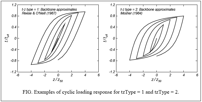
Examples of the cyclic loading response of TzSimple1 are given in the following plots. Note that the response for tzType = 2 has greater nonlinearity at smaller displacements (and hence greater hysteretic damping) and that it approaches tult more gradually (such that t/tult is still well below

EXAMPLE:

REFERENCES:

"Seismic Soil-pile-strcture interaction experiments and analysis", Boulanger, R.W., Curras, C.J., Kutter, B.L., Wilson, D.W., and Abghari, A. (1990). Jornal of Geotechnical and Geoenvironmental Engineering, ASCS, 125(9):750-759.

---

Code Developed by: Ross Boulanger, UC Davis This command is used to construct a PySimple1 uniaxial material object: