PySimple1 Material: Difference between revisions
No edit summary |
No edit summary |
||
| Line 29: | Line 29: | ||
In general the HHT algorithm is preferred over a Newmark algorithm when using this material. This is due to the numerical oscillations that can develop with viscous damping forces under transient loading with certain solution algorithms and damping ratios. | In general the HHT algorithm is preferred over a Newmark algorithm when using this material. This is due to the numerical oscillations that can develop with viscous damping forces under transient loading with certain solution algorithms and damping ratios. | ||
EQUATIONS and EXAMPLE RESPONSES: | |||
The equations describing PySimple1 behavior are described in Boulanger, R. W., Curras, C. J., | |||
Kutter, B. L., Wilson, D. W., and Abghari, A. (1999). "Seismic soil-pile-structure interaction | |||
experiments and analyses." Journal of Geotechnical and Geoenvironmental Engineering, ASCE, | |||
125(9): 750-759. Only minor changes have been made in its implementation for OpenSees. | |||
The nonlinear <math>p-y</math> behavior is conceptualized as consisting of elastic (p-ye), plastic (p-yp), and | |||
gap <math>(p-y^g)</math> components in series. Radiation damping is modeled by a dashpot on the “far-field” | |||
elastic component <math>(p-ye)</math> of the displacement rate. The gap component consists of a nonlinear | |||
closure spring (pc-yg) in parallel with a nonlinear drag spring <math>(p^d-y^g)</math>. Note that <math>y = y^e + y^p + y^g</math>, and that <math>p = p^d + p^c</math>. | |||
The plastic component has an initial range of rigid behavior between <math> -C_r p_\text{ult} < p < C_r p_\text{ult}</math> with | |||
<math>C_r</math> = the ratio of <math>p/p_\text{ult} </math> when plastic yielding first occurs in virgin loading. The rigid range of <math>p</math>, | |||
which is initially <math>2 C_r p_\text{ult}</math>, translates with plastic yielding (kinematic hardening). The rigid range | |||
of <math>p</math> can be constrained to maintain a minimum size on both the positive and negative loading | |||
sides (e.g., 25% of <math>p\text{ult}</math>), and this is accomplished by allowing the rigid range to expand or contract as necessary. Beyond the rigid range, loading of the plastic <math>(p-y^p)</math> component is | |||
described by: | |||
:<math>p = p_{\text{ult}} - (p_{\text{ult}} - p_o) \left [\frac{c * y_{50}}{c * y_{50} + | z_p - z^p_0|} \right ]^n </math> | |||
where <math>p_\text{ult}</math> = the ultimate resistance of the <math>p-y</math> material in the current loading direction, <math>p_o = p</math> at | |||
the start of the current plastic loading cycle, <math>y^p_o = y_p</math> at the start of the current plastic loading cycle, <math>c</math> = constant to control the tangent modulus at the start of plastic yielding, and n = an exponent to control sharpness of the <math>p-y^p</math> curve. | |||
[[Image:PySimple1A.gif]] | [[Image:PySimple1A.gif]] | ||
Revision as of 22:11, 22 March 2010
- Command_Manual
- Tcl Commands
- Modeling_Commands
- model
- uniaxialMaterial
- ndMaterial
- frictionModel
- section
- geometricTransf
- element
- node
- sp commands
- mp commands
- timeSeries
- pattern
- mass
- block commands
- region
- rayleigh
- Analysis Commands
- Output Commands
- Misc Commands
- DataBase Commands
This command is used to construct a PySimple1 uniaxial material object:
| uniaxialMaterial PySimple1 $matTag $soilType $pult $Y50 $Cd <$c> |
| $matTag | integer tag identifying material |
| $soilType | soilType = 1 Backbone of p-y curve approximates Matlock (1970) soft clay relation.
soilType = 2 Backbone of p-y curve approximates API (1993) sand relation. |
| $pult | Ultimate capacity of the p-y material. Note that "p" or "pult" are distributed loads [force per length of pile] in common design equations, but are both loads for this uniaxialMaterial [i.e., distributed load times the tributary length of the pile]. |
| $Y50 | Displacement at which 50% of pult is mobilized in monotonic loading. |
| $Cd | Variable that sets the drag resistance within a fully-mobilized gap as Cd*pult. |
| $c | The viscous damping term (dashpot) on the far-field (elastic) component of the displacement rate (velocity). (optional Default = 0.0). Nonzero c values are used to represent radiation damping effects |
NOTES:
In general the HHT algorithm is preferred over a Newmark algorithm when using this material. This is due to the numerical oscillations that can develop with viscous damping forces under transient loading with certain solution algorithms and damping ratios.
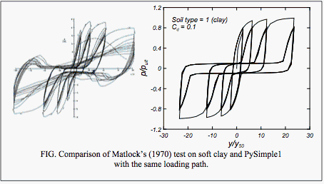
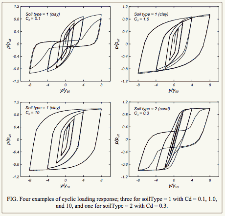
EQUATIONS and EXAMPLE RESPONSES:
The equations describing PySimple1 behavior are described in Boulanger, R. W., Curras, C. J., Kutter, B. L., Wilson, D. W., and Abghari, A. (1999). "Seismic soil-pile-structure interaction experiments and analyses." Journal of Geotechnical and Geoenvironmental Engineering, ASCE, 125(9): 750-759. Only minor changes have been made in its implementation for OpenSees.
The nonlinear <math>p-y</math> behavior is conceptualized as consisting of elastic (p-ye), plastic (p-yp), and gap <math>(p-y^g)</math> components in series. Radiation damping is modeled by a dashpot on the “far-field” elastic component <math>(p-ye)</math> of the displacement rate. The gap component consists of a nonlinear closure spring (pc-yg) in parallel with a nonlinear drag spring <math>(p^d-y^g)</math>. Note that <math>y = y^e + y^p + y^g</math>, and that <math>p = p^d + p^c</math>.
The plastic component has an initial range of rigid behavior between <math> -C_r p_\text{ult} < p < C_r p_\text{ult}</math> with <math>C_r</math> = the ratio of <math>p/p_\text{ult} </math> when plastic yielding first occurs in virgin loading. The rigid range of <math>p</math>, which is initially <math>2 C_r p_\text{ult}</math>, translates with plastic yielding (kinematic hardening). The rigid range of <math>p</math> can be constrained to maintain a minimum size on both the positive and negative loading sides (e.g., 25% of <math>p\text{ult}</math>), and this is accomplished by allowing the rigid range to expand or contract as necessary. Beyond the rigid range, loading of the plastic <math>(p-y^p)</math> component is described by:
- <math>p = p_{\text{ult}} - (p_{\text{ult}} - p_o) \left [\frac{c * y_{50}}{c * y_{50} + | z_p - z^p_0|} \right ]^n </math>
where <math>p_\text{ult}</math> = the ultimate resistance of the <math>p-y</math> material in the current loading direction, <math>p_o = p</math> at the start of the current plastic loading cycle, <math>y^p_o = y_p</math> at the start of the current plastic loading cycle, <math>c</math> = constant to control the tangent modulus at the start of plastic yielding, and n = an exponent to control sharpness of the <math>p-y^p</math> curve.
EXAMPLE:
REFERENCES:
"Seismic Soil-pile-strcture interaction experiments and analysis", Boulanger, R.w., Curras, C.J., Kutter, B.L., Wilson, D.W., and Abghari, A. (1990). Jornal of Geotechnical and Geoenvironmental Engineering, ASCS, 125(9):750-759.
Code Developed by: Ross Boulanger, UC Davis This command is used to construct a PySimple1 uniaxial material object:

