Reinforcing Steel Material: Difference between revisions
No edit summary |
No edit summary |
||
| (7 intermediate revisions by 4 users not shown) | |||
| Line 1: | Line 1: | ||
{{CommandManualMenu}} | |||
{| | |||
| style="background:red; color:black; width:800px " | | |||
'''NOTE:''' This material can lead to issues with performance in models. | |||
|} | |||
{| | {| | ||
| style="width:150px ;" | '''Contact Authors:''' || Jon Mohle M.S., P.E. | | style="width:150px ;" | '''Contact Authors:''' || Jon Mohle M.S., P.E. | ||
|- | |- | ||
| || Sashi Kunnath: | | || Sashi Kunnath: https://faculty.engineering.ucdavis.edu/kunnath/ | ||
|} | |} | ||
| Line 16: | Line 23: | ||
{| | {| | ||
| style="width:150px ;" | | | style="width:150px ;" | | ||
|- | |- | ||
| '''$matTag''' || unique material object integer tag | | '''$matTag''' || unique material object integer tag | ||
| Line 113: | Line 120: | ||
'''NOTE:''' This simulation is based on the Chang and Mander(1994) uniaxial steel model. The simulation has incorporated additional reversal memory locations to better control stress overshooting (default is 10 branches but this can be easily modified by changing the variable "LastRule_RS" within the header file "ReinforcingSteel.h"). The cycle counting method implemented in the routine achieves the same result as rainflow counting. Fatigue parameters are based on the Coffin-Manson equation for plastic strain amplitude as indicated in Figure 6a. The buckling simulations incorporated consist of a variation on Gomes and Appleton(1997) and Dhakal and Maekawa(2002). The buckling and fatigue portions of this simulation are still being further enhanced and refined. Additional buckling and fatigue options should be available in the near future. | '''NOTE:''' This simulation is based on the Chang and Mander(1994) uniaxial steel model. The simulation has incorporated additional reversal memory locations to better control stress overshooting (default is 10 branches but this can be easily modified by changing the variable "LastRule_RS" within the header file "ReinforcingSteel.h"). The cycle counting method implemented in the routine achieves the same result as rainflow counting. Fatigue parameters are based on the Coffin-Manson equation for plastic strain amplitude as indicated in Figure 6a. The buckling simulations incorporated consist of a variation on Gomes and Appleton(1997) and Dhakal and Maekawa(2002). The buckling and fatigue portions of this simulation are still being further enhanced and refined. Additional buckling and fatigue options should be available in the near future. | ||
[[File:ReinfSteel2430.png]] | |||
''Figure 1: Material Constants'' | ''Figure 1: Material Constants'' | ||
| Line 129: | Line 138: | ||
[[File:ReinfSteel2431.png]] | |||
Figure 2: Slenderness Defined | Figure 2: Slenderness Defined | ||
| Line 135: | Line 145: | ||
[[File:ReinfSteel2432.png]] | |||
Figure 3: Buckling Parameters | Figure 3: Buckling Parameters | ||
| Line 145: | Line 156: | ||
[[File:ReinfSteel2433.png]] or [[File:ReinfSteel2434.png]] | |||
| Line 152: | Line 162: | ||
[[File:ReinfSteel2435.png]] | |||
Figure 4: Effect of Sample Parameters in the Gomes and Appleton Buckling Model | Figure 4: Effect of Sample Parameters in the Gomes and Appleton Buckling Model | ||
| Line 161: | Line 172: | ||
[[File:ReinfSteel2436.png]] | |||
Figure 5: Effect of Suggested Parameters in the Dhakal and Maekawa Buckling Model | Figure 5: Effect of Suggested Parameters in the Dhakal and Maekawa Buckling Model | ||
| Line 172: | Line 184: | ||
[[File:ReinfSteel2438.png]][[File:ReinfSteel2439.png]] | |||
Figure 6a: Coffin-Manson Constants Figure 6b: Half Cycle Terms Defined | Figure 6a: Coffin-Manson Constants Figure 6b: Half Cycle Terms Defined | ||
| Line 177: | Line 190: | ||
[[File:ReinfSteel2440.png]] (1) | |||
[[File:ReinfSteel2441.png]] (2) | |||
| Line 189: | Line 200: | ||
[[File:ReinfSteel2442.png]] | |||
Figure 7: Strength Reduction | Figure 7: Strength Reduction | ||
| Line 195: | Line 207: | ||
A degrade constant, K<sub class="subscript">1</sub>, is used to describe loss in strength due to damage or other phenomenon resulting in softening due to plastic reversals. The degradation is currently assumed to have a simple linear relationship with D. This is used to correlate strength degradation to the cumulative damage factor. This linear relationship is shown in Equation 3. | A degrade constant, K<sub class="subscript">1</sub>, is used to describe loss in strength due to damage or other phenomenon resulting in softening due to plastic reversals. The degradation is currently assumed to have a simple linear relationship with D. This is used to correlate strength degradation to the cumulative damage factor. This linear relationship is shown in Equation 3. | ||
[[File:ReinfSteel2443.png]] (3) | |||
Alternately this simple linear equation can be rewritten in a way that makes the strength degradation independent of the number of half cycles to failure. Keeping the failure and degradation terms independent is convenient for calibration. Equation 3 is rewritten below utilizing the strength degradation constant C<sub class="subscript">d</sub>. | Alternately this simple linear equation can be rewritten in a way that makes the strength degradation independent of the number of half cycles to failure. Keeping the failure and degradation terms independent is convenient for calibration. Equation 3 is rewritten below utilizing the strength degradation constant C<sub class="subscript">d</sub>. | ||
[[File:ReinfSteel2444.png]] (4) | |||
The constants K<sub class="subscript">1</sub>, and C<sub class="subscript">d</sub> can be related as shown in Equation 5. | The constants K<sub class="subscript">1</sub>, and C<sub class="subscript">d</sub> can be related as shown in Equation 5. | ||
[[File:ReinfSteel2445.png]] (5) | |||
| Line 232: | Line 241: | ||
[[File:ReinfSteel2446.png]] | |||
Figure 8: Fatigue and Degradation Parameter Examples | Figure 8: Fatigue and Degradation Parameter Examples | ||
Latest revision as of 15:41, 23 July 2024
- Command_Manual
- Tcl Commands
- Modeling_Commands
- model
- uniaxialMaterial
- ndMaterial
- frictionModel
- section
- geometricTransf
- element
- node
- sp commands
- mp commands
- timeSeries
- pattern
- mass
- block commands
- region
- rayleigh
- Analysis Commands
- Output Commands
- Misc Commands
- DataBase Commands
NOTE: This material can lead to issues with performance in models. |
| Contact Authors: | Jon Mohle M.S., P.E. |
| Sashi Kunnath: https://faculty.engineering.ucdavis.edu/kunnath/ |
This command is used to construct a ReinforcingSteel uniaxial material object. This object is intended to be used in a reinforced concrete fiber section as the steel reinforcing material.
| uniaxialMaterial ReinforcingSteel $matTag $fy $fu $Es $Esh $esh $eult < -GABuck $lsr $beta $r $gama > < -DMBuck $lsr < $alpha >> < -CMFatigue $Cf $alpha $Cd > < -IsoHard <$a1 <$limit> > > |
| $matTag | unique material object integer tag |
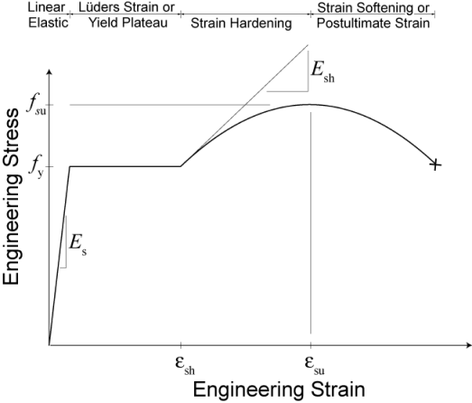
| $fy | Yield stress in tension (see Figure 1) |
| $fu | Ultimate stress in tension |
| $Es | Initial elastic tangent |
| $Esh | Tangent at initial strain hardening |
| $esh | Strain corresponding to initial strain hardening |
| $eult | Strain at peak stress |
| -GABuck | Buckling Model Based on Gomes and Appleton (1997) |
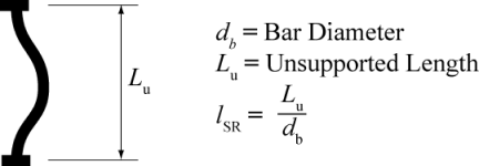
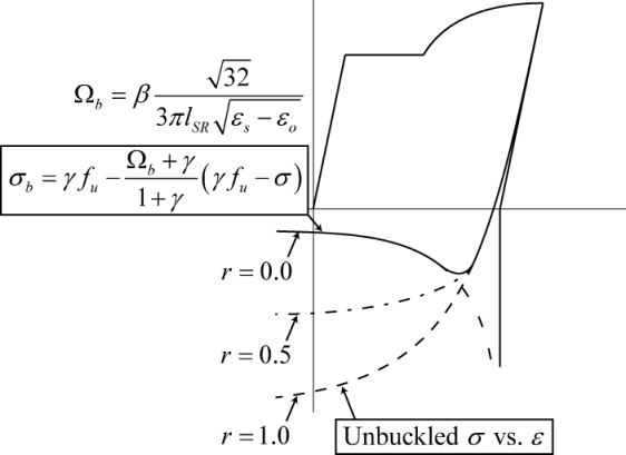
$lsr Slenderness Ratio (see Figure 2) $beta Amplification factor for the buckled stress strain curve. (see Figure 3) $r Buckling reduction factor
- r can be a real number between [0.0 and 1.0]
- r=1.0 full reduction (no buckling)
- r=0.0 no reduction
- 0.0<r<1.0 linear interpolation between buckled and unbuckled curves
$gamma Buckling constant (see Figures 3 and 4)
| -DMBuck | Buckling model based on Dhakal and Maekawa (2002) |
$lsr Slenderness Ratio (see Figure 2) $alpha Adjustment Constant usually between 0.75 and 1.0
- Default: alpha=1.0, this parameter is optional.
| -CMFatigue | Coffin-Manson Fatigue and Strength Reduction |
$Cf Coffin-Manson constant C (see Figure 5) $alpha Coffin-Manson constant a (see Figure 5) $Cd Cyclic strength reduction constant (see Figure 6 and Equation 3)
| -IsoHard | Isotropic Hardening / Diminishing Yield Plateau |
$a1 Hardening constant (default = 4.3) $limit Limit for the reduction of the yield plateau. % of original plateau length to remain (0.01 < limit < 1.0 )
- Limit =1.0, then no reduction takes place (default =0.01)
| -MPCurveParams | Menegotto and Pinto Curve Parameters see Fig 6b |
$R1 (default = 0.333) $R2 (default = 18) $R3 (default = 4)
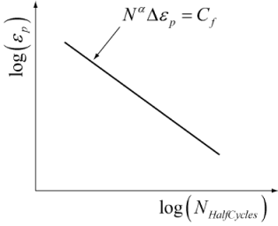
NOTE: This simulation is based on the Chang and Mander(1994) uniaxial steel model. The simulation has incorporated additional reversal memory locations to better control stress overshooting (default is 10 branches but this can be easily modified by changing the variable "LastRule_RS" within the header file "ReinforcingSteel.h"). The cycle counting method implemented in the routine achieves the same result as rainflow counting. Fatigue parameters are based on the Coffin-Manson equation for plastic strain amplitude as indicated in Figure 6a. The buckling simulations incorporated consist of a variation on Gomes and Appleton(1997) and Dhakal and Maekawa(2002). The buckling and fatigue portions of this simulation are still being further enhanced and refined. Additional buckling and fatigue options should be available in the near future.
Figure 1: Material Constants
BACKBONE CURVE: The backbone curve shown in Figure 1 is used as a bounding surface for the reinforcing bar simulation. This backbone curve is shifted as described by Chang and Mander (1994) to account for Isotropic hardening. This backbone can be obtained by utilizing simple tension test data. Within the material class, the backbone curve is transformed from engineering stress space to natural stress space (accounting for change in area as the bar is stressed.) This allows the single backbone to represent both tensile and compressive stress-strain relations. The tension and compression backbone curves are not the same in engineering stress space for this model! This transformation assumes small strain relations described by Dodd and Restrepo-Posada (1995)
The softening region (strain greater than eult), shown in Figure 1, is a localization effect due to necking and is a function of the gage length used during measurement. This geometric effect is ignored in this simulation. In this simulation, it is assumed that there is no softening in natural stress space. Because the simulation always converts back to engineering stress space, you will observe some softening in the tension response due to the reduction in area, however this will be much smaller than that shown in the original backbone curve proposed by Chang and Mander.
DIMINISHING YIELD PLATEAU: It has been observed that when a reinforcing bar is subjected to plastic strain reversals within the yield plateau, strain hardening will initiate at a lower strain that that of the same bar loaded monotonically. Additionally, isotropic hardening can result from repeated strain reversals and is commonly related to accumulated plastic strain. These two aspects of the stress-strain behavior of steel bars are somewhat related and that by shortening the yield plateau as a function of accumulated plastic strain, the model will have some capability to simulate both the diminishing yield plateau and isotropic hardening. The Chang and Mander model, on which this formulation is based, models only anisotropic hardening by shifting the backbone curves and by targeting previous reversal points on the backbone curves. By adding a component of isotropic hardening, the model has additional capabilities and is able to more accurately simulate test data.
Accumulated plastic strain is tracked within the material model for each branch, plateau adjustments are made only in the outer branches for simplicity. The plastic strain due to the backbone curve is ignored so that a monotonically loaded sample can be calibrated to a monotonic test sample more easily.
Figure 2: Slenderness Defined
Figure 3: Buckling Parameters
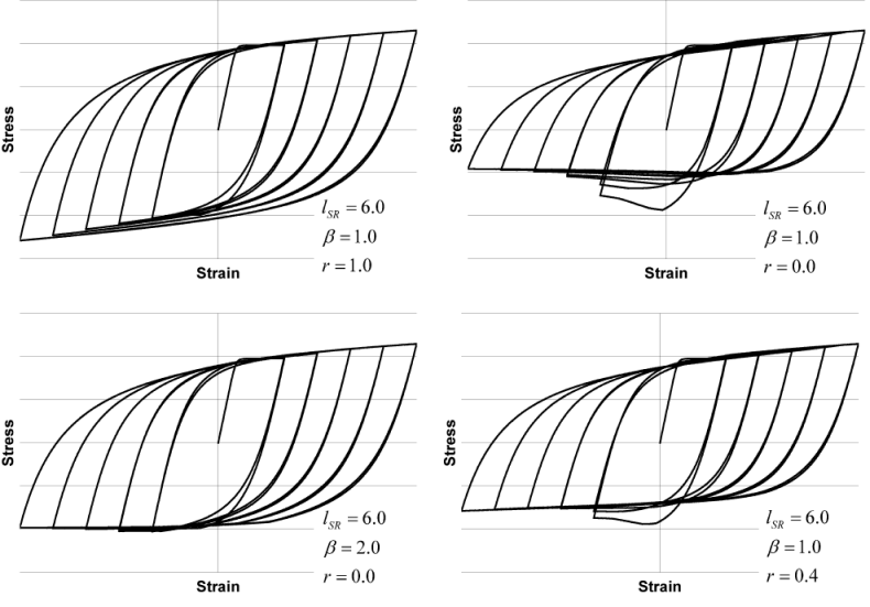
GOMES AND APPLETON BUCKLED CURVE: Figure 3 describes the use of the buckling parameters modified from Gomes and Appleton(1997). ß is an amplification factor that allows the user to scale the buckling curve. This is useful to adjust the location of the bifurcation point. The r factor is used to adjust the curve between the buckled curve and the unbuckled curve. The variable r can only be a real number between 0.0 and 1.0. The g factor is the positive stress location about which the buckling factor is initiated. This factor was introduced to avoid kinks in the reloading branch. The implementation of the g factor is shown in Figure 3. The basic idea is that the stress strain curves are reduced toward the positive stress gfsu. g should be between 0.0 and 1.0. A g of 0.0 will factor to the zero stress axis. This will usually produce a kink in the reloading curve at the zero stress location. Good results have been obtained using the following values for the buckling constants.
Figure 4 displays the buckling behavior due to the variation of the different constants. The response shown on the upper left is the unbuckled case. In each of the other cases, buckling behavior is defined by the constants shown.
Figure 4: Effect of Sample Parameters in the Gomes and Appleton Buckling Model
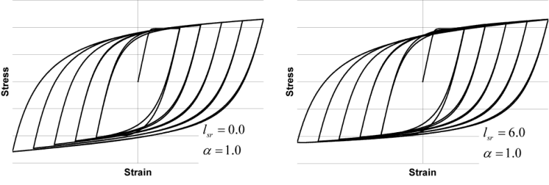
DHAKAL AND MAEKAWA BUCKLED CURVE: The buckling model described in this section is based on Dhakal and Maekawa(2002). This model takes two terms, lsr and a. lsr is the slenderness ratio as described in Figure 2 and a is an amplification factor. Dhakal and Maekawa suggest a value of a =1.0 for linear strain hardening and a =0.75 for elastic perfectly plastic material behavior. The material model in this implementation is neither linear strain hardening nor elastic perfectly plastic. However, since the material model does include strain hardening a=1.0 has been assumed as the default value. Figure 5 shows the unbuckled vs buckled stress strain response curves.
Figure 5: Effect of Suggested Parameters in the Dhakal and Maekawa Buckling Model
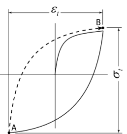
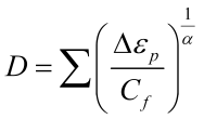
CYCLIC DEGRADATION: Cf and a are factors used to relate the number of half cycles to fracture to the half cycle plastic strain amplitude (Figure 6a). Plastic strain half cycle amplitude is defined by Equation 1. The total half cycle strain amplitude,, is shown in Figure 6b as the change in strain from reversal A to reversal B. Cf and a are used to define a cumulative damage factor, D, as described in Equation 2.
Figure 6a: Coffin-Manson Constants Figure 6b: Half Cycle Terms Defined
The cumulative damage factor is zero at no damage and 1.0 at fracture. Once a bar has been determined to have fractured, the strength is rapidly degraded to zero.
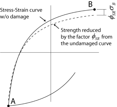
Figure 7: Strength Reduction
A degrade constant, K1, is used to describe loss in strength due to damage or other phenomenon resulting in softening due to plastic reversals. The degradation is currently assumed to have a simple linear relationship with D. This is used to correlate strength degradation to the cumulative damage factor. This linear relationship is shown in Equation 3.
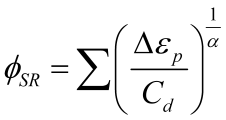
Alternately this simple linear equation can be rewritten in a way that makes the strength degradation independent of the number of half cycles to failure. Keeping the failure and degradation terms independent is convenient for calibration. Equation 3 is rewritten below utilizing the strength degradation constant Cd.
The constants K1, and Cd can be related as shown in Equation 5.
Suggested starting values have been obtained from data reported by Brown and Kunnath (2000) for bars with a slenderness of 6. Keep in mind that this experimental data is limited and additional calibration may be necessary to capture realistic behavior in a reinforcing bar embedded in concrete and influenced by other factors such as confinement.
a: 0.506
Cf: 0.26
Cd: 0.389
Sample Simulations of Degradation behavior
a is best obtained from calibration of test results. a is used to relate damage from one strain range to an equivalent damage at another strain range. This is usually constant for a material type.
Cf is the ductility constant used to adjust the number of cycles to failure. A higher value for Cf will result in a lower damage for each cycle. A higher value Cf translates to a larger number of cycles to failure.
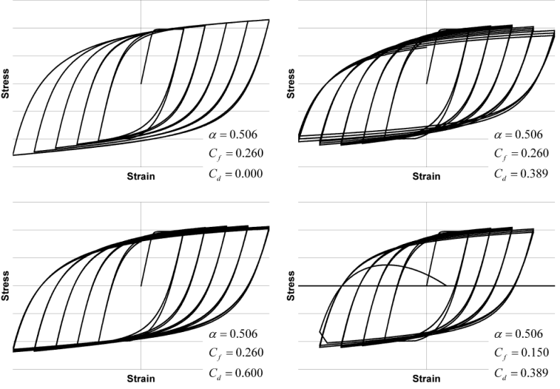
Cd is the strength reduction constant. A larger value for Cd will result in a lower reduction of strength for each cycle. The four charts shown in Figure 8 demonstrate the effect that some of the variables have on the cyclic response.
Figure 8: Fatigue and Degradation Parameter Examples
In Figure 8, the upper left response contains no strength degradation by setting the Cd variable to 0.0. The upper right response shows strength degradation due to the suggested values of Cf, a, and Cd. The response shown on the lower left demonstrates the change in the response when the suggested values of Cf and a are used with Cd=0.6. Making the value of Cd larger results in less strength reduction due to damage. The response on the lower right once again returns to the suggested values but Cf is changed to 0.15. This results in a more rapid accumulation of damage causing the bar to fail sooner. Note however that the strength degradation is unaffected by the more rapid accumulation of damage. The strength reduction and failure are not interdependent making the model easier to calibrate.
References
- Chang, G. and Mander, J. (1994). "Seismic Energy Based Fatigue Damage Analysis of Bridge Columns: Part I – Evaluation of Seismic Capacity." NCEER Technical Report 94-0006.
- Dodd, L. and Restrepo-Posada, J. (1995). "Model for Predicting Cyclic Behavior of Reinforcing Steel" J. Struct. Eng., 121(3), 433-445.
- Gomes, A., and Appleton, J. (1997). "Nonlinear Cyclic Stress-Strain Relationship of Reinforcing Bars Including Buckling." Eng. Struct., 19(10), 822–826.
- Brown, J. and Kunnath, S.K. (2000). "Low Cycle Fatigue Behavior of Longitudinal Reinforcement in Reinforced Concrete Bridge Columns." NCEER Technical Report 00-0007.
- Dhakal, R. and Maekawa, K. (2002). "Modeling for Postyield Buckled of Reinforcement" J. Struct. Eng., 128(9), 1139-1147.
