User talk:Kkolozvari: Difference between revisions
Kkolozvari (talk | contribs) |
Kkolozvari (talk | contribs) |
||
| (96 intermediate revisions by the same user not shown) | |||
| Line 1: | Line 1: | ||
== Element MVLEM == | == Element MVLEM - Multiple-Vertical-Line-Element-Model for RC Walls== | ||
{{CommandManualMenu}} | |||
Source: /usr/local/cvs/OpenSees/SRC/element/MVLEM/ | '''Developed and Implemented by:''' | ||
<span style="color:blue"> Kristijan Kolozvari<span style="color:black">, California State University, Fullerton | |||
<span style="color:blue"> Kutay Orakcal<span style="color:black">, Bogazici University, Istanbul, Turkey | |||
<span style="color:blue"> John Wallace<span style="color:black">, Univeristy of California, Los Angeles | |||
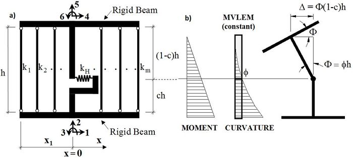
The '''MVLEM''' element command is used to generate a two-dimensional Multiple-Vertical-Line-Element-Model (MVLEM; Vulcano et al., 1988; Orakcal et al., 2004) for simulation of flexure-dominated RC wall behavior. A single model element incorporates six global degrees of freedom, three of each located at the center of rigid top and bottom beams, as illustrated in Figure 1a. The axial/flexural response of the '''MVLEM''' is simulated by a series of uniaxial elements (or macro-fibers) connected to the rigid beams at the top and bottom (e.g., floor) levels, whereas the shear response is described by a shear spring located at height ''ch'' from the bottom of the wall element (Figure 1a). Shear and flexural responses of the model element are uncoupled. The relative rotation between top and bottom faces of the wall element occurs about the point located on the central axis of the element at height ''ch'' (Figure 1b). Rotations and resulting transverse displacements are calculated based on the wall curvature, derived from section and material properties, corresponding to the bending moment at height ''ch'' of each element (Figure 1b). A value of ''c''=0.4 was recommended by Vulcano et al. (1988) based on comparison of the model response with experimental results. | |||
'''Source:''' /usr/local/cvs/OpenSees/SRC/element/MVLEM/ | |||
[[File:MVLEM.JPG|700px|thumb|center|Figure 1. a) MVLEM Element, b) MVLEM Rotations and Displacements]] | [[File:MVLEM.JPG|700px|thumb|center|Figure 1. a) MVLEM Element, b) MVLEM Rotations and Displacements]] | ||
| Line 11: | Line 21: | ||
{| | {| | ||
| style="background:yellow; color:black; width:800px" | '''Element MVLEM $eleTag $Dens $iNode $jNode $m $c -thick | | style="background:yellow; color:black; width:800px" | '''Element MVLEM $eleTag $Dens $iNode $jNode $m $c -thick {Thicknesses} -width {Widths} -rho {Reinforcing_ratios} -matConcrete {Concrete_tags} -matSteel {Steel_tags} -matShear {Shear_tag}''' | ||
|} | |} | ||
| Line 23: | Line 33: | ||
| '''$m''' || Number of element macro-fibers | | '''$m''' || Number of element macro-fibers | ||
|- | |- | ||
| '''$c''' || Location of center of rotation | | '''$c''' || Location of center of rotation from the iNode, ''c'' = 0.4 (recommended) | ||
|- | |- | ||
| ''' | | '''{Thicknesses}''' || Array of ''m'' macro-fiber thicknesses | ||
|- | |- | ||
| ''' | | '''{Widths}''' || Array of ''m'' macro-fiber widths | ||
|- | |- | ||
| ''' | | '''{Reinforcing_ratios}''' || Array of ''m'' reinforcing ratios corresponding to macro-fibers; for each fiber: rho<sub class="subscript">i</sub> = A<sub class="subscript">s,i</sub>/A<sub class="subscript">gross,i</sub> (1 < i < m) | ||
|- | |- | ||
| ''' | | '''{Concrete _tags}''' || Array of ''m'' ''uniaxialMaterial'' tags for concrete | ||
|- | |- | ||
| ''' | | '''{Steel_tags}''' || Array of ''m'' ''uniaxialMaterial'' tags for steel | ||
|- | |- | ||
| ''' | | '''{Shear_tag}''' || Tag of ''uniaxialMaterial'' for shear material | ||
|} | |} | ||
| Line 50: | Line 60: | ||
|'''Shear_Force_Deformation''' || Element shear force-deformation relationship | |'''Shear_Force_Deformation''' || Element shear force-deformation relationship | ||
|- | |- | ||
| '''Fiber_Strain''' || Vertical | | '''Fiber_Strain''' || Vertical strains in ''m'' fibers along the cross-section | ||
|- | |- | ||
| '''Fiber_Stress_Concrete''' || Vertical concrete | | '''Fiber_Stress_Concrete''' || Vertical concrete stresses in ''m'' fibers along the cross-section | ||
|- | |- | ||
| '''Fiber_Stress_Steel''' || Vertical steel | | '''Fiber_Stress_Steel''' || Vertical steel stresses in ''m'' fibers along the cross-section | ||
|} | |} | ||
| Line 71: | Line 81: | ||
'''References:''' | '''References:''' | ||
1) Orakcal K., Conte J.P., and Wallace J.W. (2004). “Flexural Modeling of Reinforced Concrete Structural Walls - Model Attributes”, ACI Structural Journal, V. 101, No. 5, pp 688-698. | |||
2) Orakcal K. and Wallace J.W. (2006). “Flexural Modeling of Reinforced Concrete Structural Walls – Experimental Verification”, ACI Structural Journal, V. 103, No. 2, pp. 196-206. | |||
3) Vulcano A., Bertero V.V., and Colotti V. (1988). “Analytical Modeling of RC Structural Walls”, Proceedings, 9th World Conference on Earthquake Engineering, V. 6, Tokyo-Kyoto, Japan, pp. 41-46. | |||
4) Orakcal K. (2004). "Nonlinear Modeling and Analysis of Slender Reinforced Concrete Walls", PhD Dissertation, Department of Civil and Environmental Engineering, University of California, Los Angeles. | |||
---- | |||
'''Example 1. Simulation of Flexural Behavior of a Slender RC Wall Specimen under Cyclic Loading using MVLEM Model''' | |||
Application of the MVLEM element for simulation of flexural response of RC walls is illustrated using the RC wall specimen RW2 tested by Thomsen and Wallace (1995). The specimen was tested under constant axial load and cyclic lateral displacement history applied at the top of the wall. Input parameters and selected output results are presented in the following sections. | |||
'''E1.1. Model Calibration''' | |||
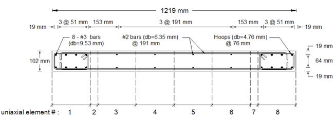
Specimen RW2 was 144 ''in'' tall, 48 ''in'' wide and 4 ''in'' thick, resulting in aspect ratio of 3.0 (slender wall). Figure E1.1 displays model discretization of the RW2 cross-section, with eight uniaxial elements defined along the length of the wall. The analytical model was discretized along wall height with 16 '''MVLEM''' elements with element heights in agreement with instrumentation provided on the specimen to allow consistent strain comparisons between model and experimental results. The material models were calibrated to match as tested material properties. Details about model calibration and experimental validation are provided by Orakcal (2004), and Orakcal and Wallace (2004). | |||
[[File:MVLEM_E1.png|650px|thumb|center|Figure E1.1. Geometry and Discretization of Wall Specimen RW2]] | |||
'''E1.2. Input Files''' | |||
Input files (.''tcl'') used to build the wall model and perform displacement-controlled analysis can be found in '''[[Media:Example 1-MVLEM.zip|Example 1. MVLEM.zip]]''': | |||
* MVLEM_RW2.tcl – model generation and definition of analysis parameters | |||
* gravity.tcl – application of gravity load | |||
* dispControl.tcl – application of lateral displacement history (run this file) | |||
* LibAnalysisStaticParameters.tcl - definition of static analysis parameters | |||
* LibGeneratePeaks.tcl - generation of displacement history | |||
'''E1.3. Analysis Results''' | |||
Flexural load-deformation responses predicted by the '''MVLEM''' model and measured during the experiment are shown on Figure E1.2. | |||
[[File:MVLEM_E2.png|450px|thumb|center|Figure E1.2. Experimental and Analytical Load versus Flexural Deformation Relationships]] | |||
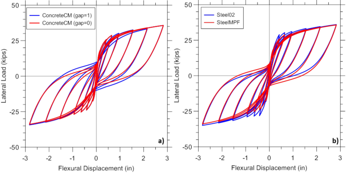
Figure E1.3 illustrates the sensitivity of analytical predictions obtained using the '''MVLEM''' to the optional gap closure parameter of the '''ConcreteCM''' model ('''-GapClose $gap''', '''LINK'''), which allows consideration of different intensities of gradual gap closure in concrete (Figure E1.3a), as well as selection of the steel material model '''SteelMPF''' versus '''Steel02''' (Figure E1.3b). It can be observed from Figure E1.3a that pinching characteristics of the response are slightly more pronounced when less gradual gap closure versus more gradual gap closure (i.e., '''gap'''=0 versus '''gap'''=1) is adopted. Figure E1.3b illustrates that the wall yield capacity as well as pinching characteristics of the behavior predicted by the '''MVLEM''' vary slightly when '''SteelMPF''' versus '''Steel02''' is used. | |||
[[File:MVLEM_E3.png|700px|thumb|center|Figure E1.3. Sensitivity of Analytical Results to Material Modeling Parameters of: a) Concrete, and b) Steel]] | |||
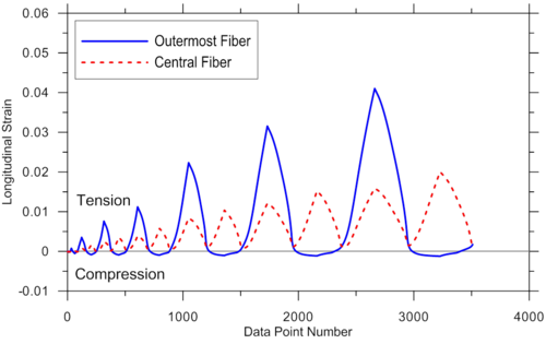
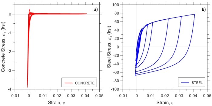
For illustration purposes, additional response predictions obtained using the '''MVLEM''' model are presented in Figure E1.4 and Figure E1.5, where analytically-predicted strain histories at the outermost and central wall fibers, and concrete and steel strain-stress relationships at the outermost fiber are presented, respectively. Responses are obtained using '''MVLEM''' recorders ''Fiber_Strain'', ''Fiber_Stress_Concrete'', and ''Fiber_Stress_Steel''. | |||
[[File:MVLEM_4.png|500px|thumb|center|Figure E1.4. Analytical Strain Histories at Outermost and Central Wall Fibers]] | |||
[[File:MVLEM_5.png|700px|thumb|center|Figure E1.5. Analytically Predicted Stress-Strain Relationships at Wall Outermost Fiber: a) Concrete, b) Steel]] | |||
== Element SFI_MVLEM - Cyclic Shear-Flexure Interaction Model for RC Walls== | |||
'''Developed and Implemented by:''' | |||
<span style="color:blue"> Kristijan Kolozvari<span style="color:black">, California State University, Fullerton | |||
== | <span style="color:blue"> Kutay Orakcal<span style="color:black">, Bogazici University, Istanbul, Turkey | ||
<span style="color:blue"> John Wallace<span style="color:black">, Univeristy of California, Los Angeles | |||
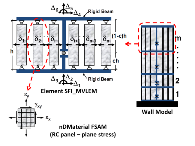
Source: /usr/local/cvs/OpenSees/SRC/element/SFI_MVLEM/ | The '''SFI_MVLEM''' command is used to construct a Shear-Flexure Interaction Multiple-Vertical-Line-Element Model (SFI-MVLEM, Kolozvari et al., 2014a, b), which captures interaction between axial/flexural and shear behavior of RC structural walls and columns under cyclic loading. The '''SFI_MVLEM''' element (Figure 1) incorporates 2-D RC panel behavior described by the Fixed-Strut-Angle-Model (nDMaterial FSAM; Ulugtekin, 2010; Orakcal et al., 2012), into a 2-D macroscopic fiber-based model (MVLEM). The interaction between axial and shear behavior is captured at each RC panel (macro-fiber) level, which further incorporates interaction between shear and flexural behavior at the '''SFI_MVLEM''' element level. | ||
'''Source:''' /usr/local/cvs/OpenSees/SRC/element/SFI_MVLEM/ | |||
[[File:SFI_MVLEM_1.png|650px|thumb|center|Figure 1. a) SFI_MVLEM Element, b) RC Panel Element (nDMaterial FSAM)]] | [[File:SFI_MVLEM_1.png|650px|thumb|center|Figure 1. a) SFI_MVLEM Element, b) RC Panel Element (nDMaterial FSAM)]] | ||
| Line 95: | Line 147: | ||
{| | {| | ||
| style="background:yellow; color:black; width:800px" | '''Element SFI_MVLEM $eleTag $iNode $jNode $m $c -thick | | style="background:yellow; color:black; width:800px" | '''Element SFI_MVLEM $eleTag $iNode $jNode $m $c -thick {Thicknesses} -width {Widths} -mat {Material_tags}''' | ||
|} | |} | ||
| Line 107: | Line 159: | ||
| '''$c''' || Location of center of rotation with from the iNode, ''c'' = 0.4 (recommended) | | '''$c''' || Location of center of rotation with from the iNode, ''c'' = 0.4 (recommended) | ||
|- | |- | ||
| ''' | | '''{Thicknesses}''' || Array of ''m'' macro-fiber thicknesses | ||
|- | |- | ||
| ''' | | '''{Widths}''' || Array of ''m'' macro-fiber widths | ||
|- | |- | ||
| ''' | | '''{Material_tags}''' || Array of ''m'' macro-fiber ''nDMaterial''<sup class="superscript">1</sup> tags | ||
|} | |} | ||
<sup class="superscript">1</sup>'''SFI_MVLEM''' element shall be used with nDMaterial '''FSAM''', which is a 2-D plane-stress constitutive relationship representing reinforced concrete panel behavior. | |||
---- | ---- | ||
| Line 126: | Line 180: | ||
|'''ShearDef''' || Element shear deformation | |'''ShearDef''' || Element shear deformation | ||
|- | |- | ||
| '''RCPanel $fibTag $Response ''' || Returns RC panel (macro-fiber) ''$Response'' for a ''$fibTag''-th panel (1 ≤ ''fibTag'' ≤ m). For available $Response-s refer to nDMaterial FSAM ('''LINK'''). | | '''RCPanel $fibTag $Response ''' || Returns RC panel (macro-fiber) ''$Response'' for a ''$fibTag''-th panel (1 ≤ ''fibTag'' ≤ m). For available ''$Response''-s refer to nDMaterial FSAM ('''LINK'''). | ||
|} | |} | ||
| Line 141: | Line 195: | ||
'''References:''' | '''References:''' | ||
1) Kolozvari K., Orakcal K., and Wallace J. W. (2015a). ”Modeling of Cyclic Shear-Flexure Interaction in Reinforced Concrete Structural Walls. I: Theory”, ASCE Journal of Structural Engineering, 141(5), 04014135 [http://dx.doi.org/10.1061/(ASCE)ST.1943-541X.0001059 doi] | |||
2) Kolozvari K., Tran T., Orakcal K., and Wallace, J.W. (2015b). ”Modeling of Cyclic Shear-Flexure Interaction in Reinforced Concrete Structural Walls. II: Experimental Validation”, ASCE Journal of Structural Engineering, 141(5), 04014136 [http://dx.doi.org/10.1061/(ASCE)ST.1943-541X.0001083 doi] | |||
3) Kolozvari K. (2013). “Analytical Modeling of Cyclic Shear-Flexure Interaction in Reinforced Concrete Structural Walls”, PhD Dissertation, University of California, Los Angeles. | |||
---- | |||
'''Example 1. Simulation of Shear-Flexural Behavior of a Medium-Rise RC Wall Specimen under Cyclic Loading using the SFI-MVLEM Model''' | |||
The behavior of RC wall specimen RW-A15-P10-S78 (Tran and Wallace, 2012) tested under constant axial load and cyclic lateral displacement history applied at the top of the wall is predicted using the '''SFI_MVLEM''' model. The input parameters and output results are presented in the following sections. | |||
'''E1.1. Model Calibration''' | |||
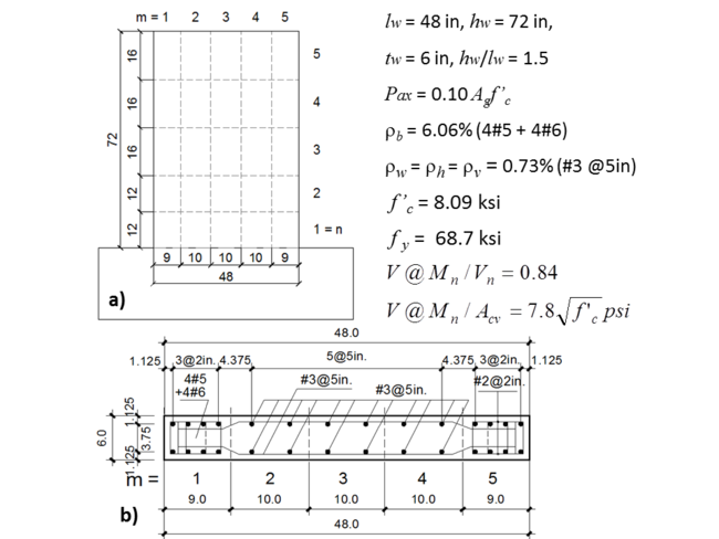
Basic properties of the specimen with model discretization are shown on Figure E1.1. Detailed information about the test specimen can be found in paper by Tran and Wallace (2012), whereas details of model calibration are provided by Kolozvari (2013) and Kolozvari et al. (2015b). | |||
[[File:Example2_1.png|650px|thumb|center|Figure E1.1. Model discretization: a) Plan view, b) Cross-section]] | |||
'''E1.2. Input Files''' | |||
Input files (.''tcl'') used to build the wall model and perform displacement-controlled analysis can be found in '''[[Media:Example 1-SFI_MVLEM.zip|Example 1. SFI_MVLEM.zip]]''': | |||
* SFI_MVLEM_SP4.tcl – model generation and definition of analysis parameters | |||
* gravity.tcl – application of gravity load | |||
* dispControl.tcl – application of lateral displacement history (run this file) | |||
* LibAnalysisStaticParameters.tcl - definition of static analysis parameters | |||
* LibGeneratePeaks.tcl - generation of displacement history | |||
'''E1.3. Analysis Results''' | |||
The following sub-section presents analytical results obtained for the test specimen described above, using the input files provided. The results include global wall responses (compared against experimental results), model element responses, and individual RC panel (macro-fiber) responses. | |||
''E1.3.1. Global Wall Responses'' | |||
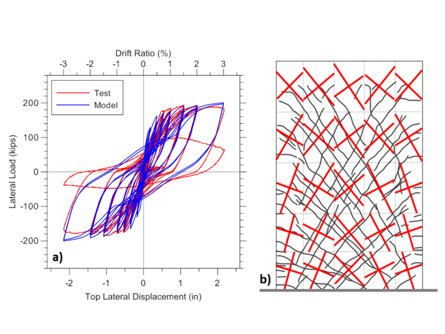
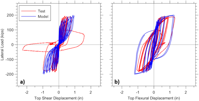
Analytical and experimental lateral load versus top total displacement responses and wall cracking patterns are presented on Figure E1.2, whereas lateral load versus flexural and shear deformations are shown on Figure E1.3. Total top displacement is obtained from the top node, shear force is recorded using ''globalForce'' element recorder, total shear displacement is obtained using ''shearDef'' element recorder and crack orientations are obtained using ''RCPanel'' and ''cracking_angles'' element recorders. | |||
[[File:Example2_2.png|650px|thumb|center|Figure E1.2. Wall responses: a) Load versus Top Displacement Behavior, b) Cracking Patterns]] | |||
[[File:Example2_3.png|650px|thumb|center|Figure E1.3. Load versus Deformation Behavior for: a) Flexure, b) Shear]] | |||
''E1.3.2. Model Element Responses'' | |||
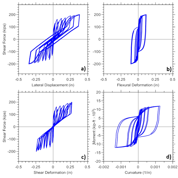
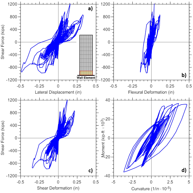
Figure E1.4 plots lateral load versus total, flexural and shear displacement responses, as well as moment versus curvature relationship, obtained from the analysis for the bottom wall model element. Responses are recorded using ''globalForce'', ''ShearDef'', and ''Curvature'' element recorders. | |||
[[File:Example2_31.png|650px|thumb|center|Figure E1.4. Model Element Responses: a) Shear Force vs. Total Deformation, b) Shear force vs. Flexural Deformation, c) Shear Force vs. Shear Deformation, d) Moment vs. Curvature]] | |||
''E1.3.3. Reinforced Concrete Panel Responses'' | |||
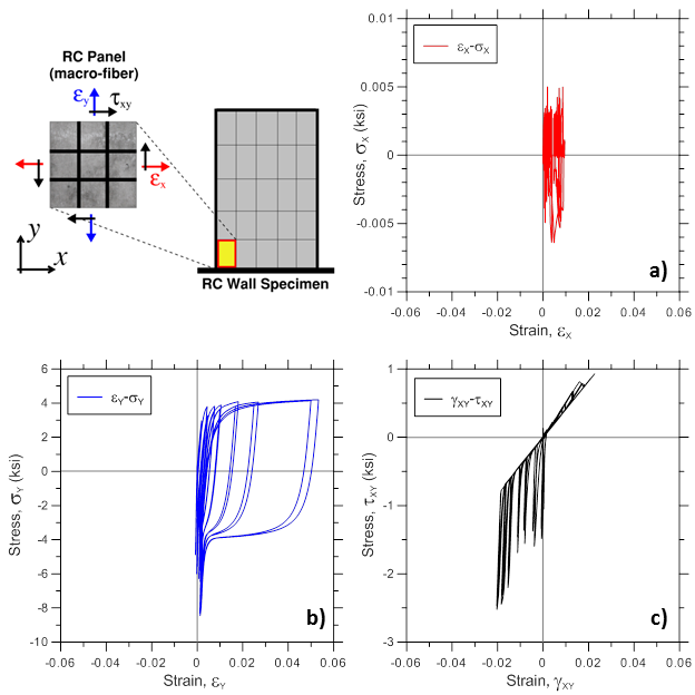
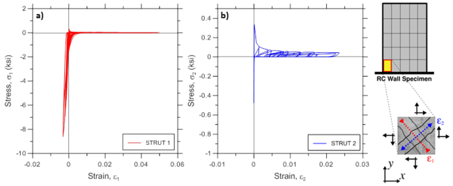
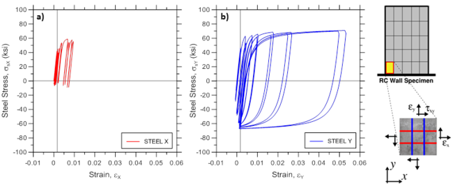
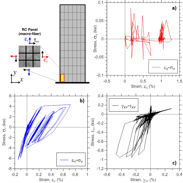
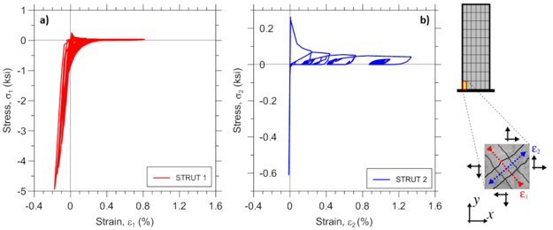
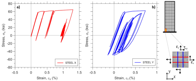
Various stress-strain responses for an individual boundary panel element (outermost macro-fiber) within the bottommost wall element are presented, including total (resultant) stress vs. strain relationships in the ''xy'' plane (Figure E1.5; element ''RCPanel'' recorders: ''panel_strain'' and ''panel_stress''), stress-strain relationships along the two concrete struts (Figure E1.6; element ''RCPanel'' recorders: ''strain_stress_concrete1'' and ''strain_stress_concrete2''), and stress-strain relationship along horizontal and vertical steel reinforcement (Figure E1.7; element ''RCPanel'' recorders: ''strain_stress_steelX'' and ''strain_stress_steelY''). | |||
[[File:Example2_4.png|650px|thumb|center|Figure E1.5. Panel Total Stress vs. Strain Responses: a) Axial-Horizontal, b) Axial-Vertical, c) Shear]] | |||
[[File:Example2_5.png|650px|thumb|center|Figure E1.6. Predicted Stress-Strain Behavior for Concrete: a) Strut 1, b) Strut 2]] | |||
[[File:Example2_6.png|650px|thumb|center|Figure E1.7. Predicted Stress-Strain Behavior for Steel: a) Horizontal (X), b) Vertical (Y)]] | |||
---- | |||
'''Example 2. Dynamic Analysis of a Coupled Wall-Frame System''' | |||
This example illustrates application of the '''SFI_MVLEM''' wall model for nonlinear dynamic analysis. Analytical model of a coupled wall-frame building system was generated and analyzed under a single ground motion time-history. Brief description of the building characteristics and the analytical model are provided in the following sections. | |||
'''E2.1. Building Description''' | |||
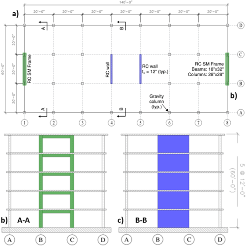
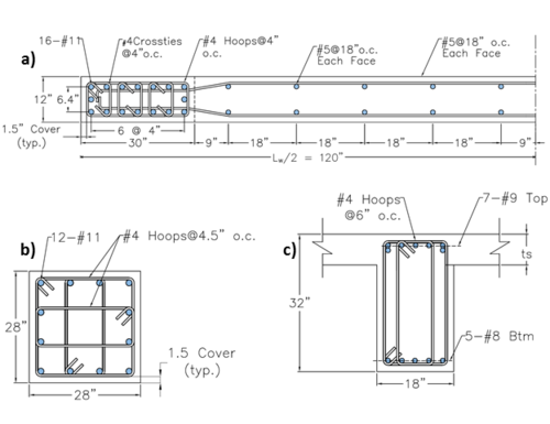
Plan and elevation/section views of the considered building are shown in Figure E2.1. The building footprint is 140 ''ft'' × 60 ''ft'', with 20 ''ft'' long spans. Analysis is conducted for shaking in the transverse direction only, where the lateral-force-resisting elements include two identical one-bay frames located at the building perimeter (axis 1 and 8, Figure E2.1a) and two identical walls located near the center of the building (axis 4 and 5, Figure E2.1a). Structural design is performed for a residential building (I=1.0, risk category I, design category D; ASCE 7-10 S11.5 and S11.6) for uniformly distributed dead load of 150 ''psf'' and live load of 40 ''psf'' (ASCE 7-10, Table 4-1), as well as the earthquake lateral loading obtained using Equivalent Lateral Force Procedure of ASCE 7-10 (S12.8). The frame was designed to resist 25% of the earthquake lateral load (Dual System, ASCE 7-10). Concrete compressive strength of f’<sub class="subscript">c</sub> = 5,000 ''psi'' and reinforcing steel (both longitudinal and transversal reinforcement) with yield strength f<sub class="subscript">y</sub> = 60,000 ''psi'' were used. Based on the structural design, cross-section dimensions of 12 ''in'' × 240 ''in'' (walls), 18 ''in'' × 32 ''in'' (beams; width × depth), and 28 ''in'' × 28 ''in'' (columns) were adopted. Cross-sections of structural elements with the reinforcement detailing are provided in Figure E2.2. | |||
[[File:SFI_MVLEM_E2_1.png|500px|thumb|center|Figure E2.1. Building Views: a) Plan View, b) Frame Elevation, c) Wall Elevation]] | |||
[[File:SFI_MVLEM_E2_2.png|500px|thumb|center|Figure E2.2. Member Cross-Sections: a) Walls, b) Columns, c) Beams]] | |||
'''E2.2. Analytical Model Description''' | |||
Due to building symmetry and applied direction of the ground motion, a two-dimensional model consisting of one frame and one wall (Figure E2.3) is used to simulate the building behavior. The gravity system is not included in the model (ASCE 7-10) and the assumption of a rigid diaphragm is implemented within each story level. Tributary mass is assigned at the element nodes at each story level at locations of axes of the vertical elements (i.e., wall and columns), whereas gravity load (dead and live) was assigned according to corresponding tributary areas as either nodal load at wall-element nodes of each story or uniformly distributed load along the beams of the frame. | |||
As show on Figure E2.3, the RC wall is modeled using ten equal-length '''SFI_MVLEM''' elements along the wall height (i.e., two elements per story height). Wall discretization in horizontal direction was performed using six macro-fibers to represent the wall cross section, where two outer macro-fibers were used to represent the confined wall boundaries and the remaining four represent the unconfined wall web. Material models for steel and concrete are calibrated based on adopted material strengths to represent the behavior of confined and unconfined concrete and reinforcing steel. | |||
RC frame elements (i.e., beams and columns) are modeled using elastic beam-column elements by assuming the location of plastic hinges at the faces of beam-column joints (Figure E2.3a), the behavior of which was simulated using zero-length elements at locations of hinges and the elasto-plastic moment-rotation hysteretic model (Modified Ibarra Krawinkler Deterioration Model; Lignos and Krawinkler, 2011), with modeling parameters adopted according to beam and column flexural capacities and the ASCE 41 backbone relationships (Figure E2.3b). The reduction of flexural stiffness after cracking was considered using stiffness modifiers for elastic portions of beam and column elements according to ASCE 41 (Table 6.5). | |||
'''E2.3. Input Files''' | |||
Input files (.''tcl'') used to build the model of a 5-story wall-frame system and perform gravity and dynamic analysis can be found in '''[[Media:Example 2-SFI_MVLEM.zip|Example 2. SFI_MVLEM.zip]]''': | |||
* 5storyWF_SFI.tcl – model generation, definition of analysis parameters, gravity analysis | |||
* Modal.tcl – modal analysis | |||
* Dynamic.tcl – application of earthquake acceleration time-history (run this file) | |||
* MCEScaledEQ1X.acc – earthquake acceleration time history file | |||
* DisplayModel2D.tcl - display 2D model | |||
* DisplayPlane.tcl - display plane | |||
[[File:SFI_MVLEM_E2_3.png|650px|thumb|center|Figure E2.3. Analytical Model of Building System: a) Modeling Approach, b) Plastic Hinge Model]] | |||
'''E2.4. Dynamic Analysis Results''' | |||
Results obtained using analytical model of the building described in the previous section are presented, including modal properties of the structure, wall global (i.e., lateral deformations, drifts, shear force, moments) and local (i.e., vertical strains and rotations) responses. Responses of the structural elements comprising the RC frame are not considered. | |||
''E2.4.1. Dynamic Properties'' | |||
First two building fundamental periods and mode shapes are presented in Figure E2.4. | |||
[[File:SFI_MVLEM_E2_4.png|800px|thumb|center|Figure E2.4. Mode Shapes: a) 1st Mode, b) 2nd Mode]] | |||
''E2.4.2. Time-history Responses'' | |||
Time histories of ground motion acceleration, wall top nodal displacement, and wall base shear force (bottom wall node reaction) are presented in Figure 2.5; the responses are obtained using ''globalForce'' and ''Reactions'' node recorders. | |||
[[File:SFI_MVLEM_E2_5.png|500px|thumb|center|Figure E2.5. Global Building Responses]] | |||
''E2.4.3. Maximum Global Responses over the Wall Height'' | |||
Maximum envelopes of wall lateral displacements and interstory drifts, and shear force and bending moment are presented in Figure E2.6 and Figure E2.7, respectively. Wall lateral displacements and drifts are obtained using corresponding node recorders, ''disp'' and ''drift'', whereas shear force and bending moments over the wall height are recorded using element recorders ''globalForce''. | |||
[[File:SFI_MVLEM_E2_6.png|625px|thumb|center|Figure E2.6. Maximum Deformation Responses: a) Lateral Displacements, b) Interstory Drifts]] | |||
[[File:SFI_MVLEM_E2_7.png|625px|thumb|center|Figure E2.7. Maximum Shear Force and Bending Moment over Wall Height]] | |||
''E2.4.4. Bottom Wall Element Responses'' | |||
Figure E2.8 plots the responses of the bottom wall element, including lateral load versus total, flexural and shear displacement, and moment versus curvature relationship obtained from the dynamic analysis. Note that wall element shear displacement and curvature time-histories are obtained using '''SFI_MVLEM''' element recorders ''ShearDef'' and ''Curvature'', respectively, whereas shear force and bending moment are recorded using element recorder ''globalForce''. | |||
[[File:SFI_MVLEM_E2_8.png|650px|thumb|center|Figure E2.8. Model Element Responses: a) Lateral Load vs. Displacement, b) Lateral Load vs. Flexural Deformation, c) Lateral Load vs. Shear Deformation, d) Moment vs. Curvature]] | |||
''E2.4.5. Single RC Panel Responses'' | |||
Analytically-predicted strain-stress responses of a single RC panel (macro-fiber) located at the left wall boundary of the bottom wall element are presented. Global panel stress-strain relationships presented on Figure E2.9 are obtained using element recorder ''RCPanel'' with commands ''panel_strain'' and ''panel_stress''; the uniaxial behavior of concrete along the two concrete struts presented on Figure E2.10 are recorded using ''strain_stress_concrete1'' and ''strain_stress_concrete2'' commands; uniaxial stress-strain behavior of horizontal and vertical reinforcing steel presented on Figure E2.11 are obtained using ''strain_stress_steelX'' and ''strain_stress_steelY'' commands. Other panel responses described in Section 3 could be plotted in a similar manner. | |||
[[File:SFI_MVLEM_E2_9.png|650px|thumb|center|Figure E2.9. Panel Total Stress vs. Strain Responses: a) Axial-Horizontal, b) Axial-Vertical, c) Shear]] | |||
[[File:SFI_MVLEM_E2_10.png|625px|thumb|center|Figure E2.10. Predicted Stress-Strain Behavior for Concrete: a) Strut 1, b) Strut 2]] | |||
[[File:SFI_MVLEM_E2_11.png|625px|thumb|center|Figure E2.11. Predicted Stress-Strain Behavior for Steel: a) Horizontal (X), b) Vertical (Y)]] | |||
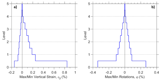
Finally, vertical profiles of maximum vertical strains (Figure E2.12a) are obtained using element recorder with ''RCPanel'' and ''panel_strain'' recorder commands, whereas maximum wall rotations over the wall height (Figure E2.12b) are derived from element ''Curvature'' recorder. Similarly, the distribution of other wall responses could be plotted over the wall height (e.g., shear deformations, etc.). | |||
[[File:SFI_MVLEM_E2_12.png|625px|thumb|center|Figure E2.12. Local Responses - Vertical Profiles of Maximum: a) Vertical Strains, b) Rotations]] | |||
== uniaxialMaterial SteelMPF - Steel Material Model by Menegotto and Pinto (1973) extended by Filippou et al. (1983) == | |||
'''Developed and Implemented by:''' | |||
<span style="color:blue"> Kristijan Kolozvari<span style="color:black">, California State University, Fullerton | |||
<span style="color:blue"> Kutay Orakcal<span style="color:black">, Bogazici University, Istanbul, Turkey | |||
== | <span style="color:blue"> John Wallace<span style="color:black">, Univeristy of California, Los Angeles | ||
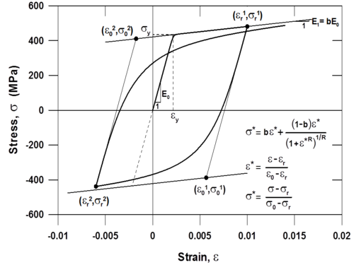
This command is used to construct a uniaxialMaterial '''SteelMPF''', which represents the well-known uniaxial constitutive nonlinear hysteretic material model for steel proposed by Menegotto and Pinto (1973), and extended by Filippou et al. (1983) to include isotropic strain hardening effects. The relationship is in the form of curved transitions (Figure 1), each from a straight-line asymptote with slope | This command is used to construct a uniaxialMaterial '''SteelMPF''', which represents the well-known uniaxial constitutive nonlinear hysteretic material model for steel proposed by Menegotto and Pinto (1973), and extended by Filippou et al. (1983) to include isotropic strain hardening effects. The relationship is in the form of curved transitions (Figure 1), each from a straight-line asymptote with slope E<sub class="subscript">0</sub> (modulus of elasticity) to another straight-line asymptote with slope E<sub class="subscript">1</sub> = bE<sub class="subscript">0</sub> (yield modulus) where ''b'' is the strain hardening ratio. The curvature of the transition curve between the two asymptotes is governed by a cyclic curvature parameter ''R'', which permits the Bauschinger effect to be represented, and is dependent on the absolute strain difference between the current asymptote intersection point and the previous maximum or minimum strain reversal point depending on whether the current strain is increasing or decreasing, respectively. The strain and stress pairs (ε<sub class="subscript">r</sub>,σ<sub class="subscript">r</sub>) and (ε<sub class="subscript">0</sub>,σ<sub class="subscript">0</sub>) shown on Figure 1 are updated after each strain reversal. | ||
Source: /usr/local/cvs/OpenSees/SRC/material/uniaxial/ | '''Source:''' /usr/local/cvs/OpenSees/SRC/material/uniaxial/ | ||
[[File:SteelMPF.png|500px|thumb|center|Figure 1. Constitutive Model for Steel (Menegotto and Pinto, 1973)]] | [[File:SteelMPF.png|500px|thumb|center|Figure 1. Constitutive Model for Steel (Menegotto and Pinto, 1973)]] | ||
| Line 171: | Line 352: | ||
{| | {| | ||
| style="width:150px" | '''$mattag''' || Unique | | style="width:150px" | '''$mattag''' || Unique ''uniaxialMaterial'' tag | ||
|- | |- | ||
|'''$fyp''' || Yield strength in tension (positive loading direction) | |'''$fyp''' || Yield strength in tension (positive loading direction) | ||
|- | |- | ||
| ''' | | '''$fyn''' || Yield strength in compression (negative loading direction) | ||
|- | |- | ||
| '''$E0''' || Initial tangent modulus | | '''$E0''' || Initial tangent modulus | ||
| Line 181: | Line 362: | ||
| '''$bp''' || Strain hardening ratio in tension (positive loading direction) | | '''$bp''' || Strain hardening ratio in tension (positive loading direction) | ||
|- | |- | ||
| '''$bn''' || Strain hardening ratio in compression ( negative loading direction) | | '''$bn''' || Strain hardening ratio in compression (negative loading direction) | ||
|- | |- | ||
| '''$R0''' || Initial value of the curvature parameter R (R0 = 20 recommended) | | '''$R0''' || Initial value of the curvature parameter R (R0 = 20 recommended) | ||
| Line 202: | Line 383: | ||
'''Discussion:''' | '''Discussion:''' | ||
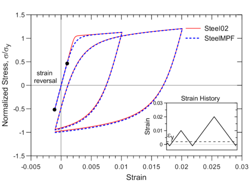
Although the Menegotto-Pinto model is already available in OpenSees (e.g., Steel02), the formulation of SteelMPF | Although the Menegotto-Pinto model is already available in OpenSees (e.g., '''Steel02'''), the formulation of '''SteelMPF''' introduces several distinctive features compared to existing models. For example, the model allows definition of different yield stress values and strain hardening ratios for tension and compression, and it considers degradation of cyclic curvature parameter ''R'' for strain reversals in both pre- and post- yielding regions, which could produce more accurate predictions of yield capacity for some RC wall specimens (see '''LINK''' Example 1), whereas '''Steel02''' considers the degradation in post-yielding region only. Strain-stress relationships obtained using '''SteelMPF''' and '''Steel02''' are compared in Figure 2 for a strain history that includes strain reversals at strain values equal to one-half of the yield strain (e.i., <math>\epsilon</math><sub class="subscript">r</sub> = ±0.001 = <math>\epsilon</math><sub class="subscript">y/2</sub>). The model also allows calibration of isotropic hardening parameters through optional input variables ''a<sub class="subscript">3</sub>'' and ''a<sub class="subscript">4</sub>'', and uses default values of ''a<sub class="subscript">3</sub>'' = 0.01 and ''a<sub class="subscript">4</sub>'' = 7.0 as calibrated by Filippou et al. (1983) based on test results. To disregard isotropic strain hardening behavior in '''SteelMPF''', parameter ''a<sub class="subscript">3</sub>'' needs to be assigned a zero value (''a<sub class="subscript">3</sub>'' = 0.0). | ||
[[File:SteelMPF_1.png|500px|thumb|center|Figure 2. Comparison of Steel02 and SteelMPF]] | [[File:SteelMPF_1.png|500px|thumb|center|Figure 2. Comparison of Steel02 and SteelMPF]] | ||
| Line 209: | Line 390: | ||
'''References:''' | '''References:''' | ||
1) Filippou F.C., Popov, E.P., and Bertero, V.V. (1983). "Effects of Bond Deterioration on Hysteretic Behavior of Reinforced Concrete Joints". Report EERC 83-19, Earthquake Engineering Research Center, University of California, Berkeley. | |||
2) Menegotto, M., and Pinto, P.E. (1973). Method of analysis of cyclically loaded RC plane frames including changes in geometry and non-elastic behavior of elements under normal force and bending. Preliminary Report IABSE, vol 13. | |||
== uniaxialMaterial ConcreteCM - Complete Concrete Model by Chang and Mander (1994)== | |||
'''Developed and Implemented by:''' | |||
<span style="color:blue"> Kristijan Kolozvari<span style="color:black">, California State University, Fullerton | |||
<span style="color:blue"> Kutay Orakcal<span style="color:black">, Bogazici University, Istanbul, Turkey | |||
== | <span style="color:blue"> John Wallace<span style="color:black">, Univeristy of California, Los Angeles | ||
This command is used to construct a uniaxialMaterial '''ConcreteCM''', which is a uniaxial hysteretic constitutive model for concrete developed by Chang and Mander (1994). This model is a refined, rule-based, generalized, and non-dimensional constitutive model that allows calibration of the monotonic and hysteretic material modeling parameters, and can simulate the hysteretic behavior of confined and unconfined, ordinary and high-strength concrete, in both cyclic compression and tension (Figure 1). The model addresses important behavioral features, such as continuous hysteretic behavior under cyclic compression and tension, progressive stiffness degradation associated with smooth unloading and reloading curves at increasing strain values, and gradual crack closure effects. Details of the model are available in the report by Chang and Mander (1994) | This command is used to construct a uniaxialMaterial '''ConcreteCM''', which is a uniaxial hysteretic constitutive model for concrete developed by Chang and Mander (1994). This model is a refined, rule-based, generalized, and non-dimensional constitutive model that allows calibration of the monotonic and hysteretic material modeling parameters, and can simulate the hysteretic behavior of confined and unconfined, ordinary and high-strength concrete, in both cyclic compression and tension (Figure 1). The model addresses important behavioral features, such as continuous hysteretic behavior under cyclic compression and tension, progressive stiffness degradation associated with smooth unloading and reloading curves at increasing strain values, and gradual crack closure effects. Details of the model are available in the report by Chang and Mander (1994). | ||
[[File:ConcreteCM_0.png|500px|thumb|center|Figure 1. Hysteretic Constitutive Model for Concrete by Chang and Mander (1994)]] | [[File:ConcreteCM_0.png|500px|thumb|center|Figure 1. Hysteretic Constitutive Model for Concrete by Chang and Mander (1994)]] | ||
The Chang and Mander (1994) model successfully generates continuous hysteretic stress-strain relationships with slope continuity for confined and unconfined concrete in both compression and tension. The compression envelope curve of the model is defined by the initial tangent slope, ( | The Chang and Mander (1994) model successfully generates continuous hysteretic stress-strain relationships with slope continuity for confined and unconfined concrete in both compression and tension. The compression envelope curve of the model is defined by the initial tangent slope, (E<sub class="subscript">c</sub>), the peak coordinate (<math>\epsilon</math>'<sub class="subscript">c</sub>, f'<sub class="subscript">c</sub>), a parameter (r<sub class="subscript">c</sub>) from Tsai’s (1988) equation defining the shape of the envelope curve, and a parameter (<math>\epsilon</math><sup class="superscript">-</sup><sub class="subscript">cr</sub>) to define normalized (with respect to <math>\epsilon</math>'<sub class="subscript">c</sub>) strain where the envelope curve starts following a straight line, until zero compressive stress is reached at the spalling strain, <math>\epsilon</math><sub class="subscript">sp</sub>. These parameters can be controlled based on specific experimental results for a refined calibration of the compression envelope (Figure 2). Chang and Mander (1994) proposed empirical relationships for parameters E<sub class="subscript">c</sub>, <math>\epsilon</math>'<sub class="subscript">c</sub>, and r<sub class="subscript">c</sub> for unconfined concrete with compressive strength f'<sub class="subscript">c</sub>, based on review of previous research. Parameters f'<sub class="subscript">c</sub>, <math>\epsilon</math>'<sub class="subscript">c</sub>, E<sub class="subscript">c</sub>, r<sub class="subscript">c</sub>, and <math>\epsilon</math><sup class="superscript">-</sup><sub class="subscript">cr</sub> can also be calibrated to represent the stress-strain behavior of confined concrete in compression, to follow the constitutive relationships for confined concrete proposed by Mander et al (1988) or similar. | ||
[[File:ConcreteCM_1.png|500px|thumb|center|Figure 2. Compression and Tension Envelope Curves]] | [[File:ConcreteCM_1.png|500px|thumb|center|Figure 2. Compression and Tension Envelope Curves]] | ||
The shape of the tension envelope curve in the model is the same as that of the compression envelope; however, the tension envelope curve is shifted to a new origin that is based on the unloading strain from the compression envelope (Figure 2). As well, the strain ductility experienced previously on the compression envelope is also reflected on the tension envelope. The parameters associated with the tension envelope curve include the tensile strength of concrete ( | The shape of the tension envelope curve in the model is the same as that of the compression envelope; however, the tension envelope curve is shifted to a new origin that is based on the unloading strain from the compression envelope (Figure 2). As well, the strain ductility experienced previously on the compression envelope is also reflected on the tension envelope. The parameters associated with the tension envelope curve include the tensile strength of concrete (f<sub class="subscript">t</sub>), the monotonic strain at tensile strength (<math>\epsilon</math><sub class="subscript">t</sub>), a parameter (r<sub class="subscript">t</sub>) from Tsai’s (1988) equation defining the shape of the tension envelope curve, and a parameter (<math>\epsilon</math><sup class="superscript">+</sup><sub class="subscript">cr</sub>) to define normalized (with respect to <math>\epsilon</math><sub class="subscript">t</sub>) strain where the tension envelope curve starts following a straight line, until zero tensile stress is reached at a strain of <math>\epsilon</math><sub class="subscript">crk</sub>. These parameters can also be controlled and calibrated based on specific experimental results or empirical relations proposed by other researchers (e.g., Belarbi and Hsu, 1994) to model the behavior of concrete in tension and the tension stiffening phenomenon. Concrete experiencing tension stiffening can be considered not to crack completely; that is, a large value for parameter <math>\epsilon</math><sup class="superscript">+</sup><sub class="subscript">cr</sub> (e.g., 10000) can be defined. | ||
Source: /usr/local/cvs/OpenSees/SRC/material/uniaxial/ | Source: /usr/local/cvs/OpenSees/SRC/material/uniaxial/ | ||
| Line 245: | Line 426: | ||
| style="width:150px" | '''$mattag''' || Unique ''uniaxialMaterial'' tag | | style="width:150px" | '''$mattag''' || Unique ''uniaxialMaterial'' tag | ||
|- | |- | ||
|'''$fpcc''' || Compressive strength | |'''$fpcc''' || Compressive strength (f'<sub class="subscript">c</sub>) | ||
|- | |- | ||
| '''$epcc''' || Strain at compressive strength | | '''$epcc''' || Strain at compressive strength (<math>\epsilon</math>'<sub class="subscript">c</sub>) | ||
|- | |- | ||
| '''$Ec''' || Initial tangent modulus | | '''$Ec''' || Initial tangent modulus (E<sub class="subscript">c</sub>) | ||
|- | |- | ||
| '''$rc''' || Shape parameter in Tsai’s equation defined for compression | | '''$rc''' || Shape parameter in Tsai’s equation defined for compression (r<sub class="subscript">c</sub>) | ||
|- | |- | ||
| '''$xcrn''' || Non-dimensional critical strain on compression envelope (where the envelope curve starts following a straight line) | | '''$xcrn''' || Non-dimensional critical strain on compression envelope (<math>\epsilon</math><sup class="superscript">-</sup><sub class="subscript">cr</sub>, where the envelope curve starts following a straight line) | ||
|- | |- | ||
| '''$ft''' || Tensile strength | | '''$ft''' || Tensile strength (f<sub class="subscript">t</sub>) | ||
|- | |- | ||
| '''$rt''' || Shape parameter in Tsai’s equation defined for tension | | '''$rt''' || Shape parameter in Tsai’s equation defined for tension (r<sub class="subscript">t</sub>) | ||
|- | |- | ||
| '''$xcrp''' || Non-dimensional critical strain on tension envelope (where the envelope curve starts following a straight line – large value [e.g., 10000] recommended when tension stiffening is considered) | | '''$xcrp''' || Non-dimensional critical strain on tension envelope (<math>\epsilon</math><sup class="superscript">+</sup><sub class="subscript">cr</sub>, where the envelope curve starts following a straight line – large value [e.g., 10000] recommended when tension stiffening is considered) | ||
|- | |- | ||
| '''<-GapClose $gap>''' || '''gap''' = 0, less gradual gap closure (default); '''gap''' = 1, more gradual gap closure | | '''<-GapClose $gap>''' || '''gap''' = 0, less gradual gap closure (default); '''gap''' = 1, more gradual gap closure | ||
| Line 276: | Line 457: | ||
'''Discussion:''' | '''Discussion:''' | ||
An optional input parameter '''gap''' is introduced in the '''ConcreteCM''' model implemented in OpenSees for providing the users with the opportunity to control the intensity of gap closure in the stress-strain behavior of concrete, which in-turn influences the level of pinching in the lateral load-displacement behavior of a RC wall. The original Chang and Mander (1994) model adopts a non-zero tangent stiffness at zero stress level upon unloading from the tension envelope, which is represented by gap = 1 in '''ConcreteCM'''. Using '''gap''' = 0 (default) produces less gradual gap closure, since it assumes zero tangent stiffness at zero stress level upon unloading from the tension envelope, and is suitable for most analyses. Figure 4 illustrates the effect of plastic stiffness upon unloading from tension envelope ( | An optional input parameter '''gap''' is introduced in the '''ConcreteCM''' model implemented in OpenSees for providing the users with the opportunity to control the intensity of gap closure in the stress-strain behavior of concrete, which in-turn influences the level of pinching in the lateral load-displacement behavior of a RC wall. The original Chang and Mander (1994) model adopts a non-zero tangent stiffness at zero stress level upon unloading from the tension envelope, which is represented by gap = 1 in '''ConcreteCM'''. Using '''gap''' = 0 (default) produces less gradual gap closure, since it assumes zero tangent stiffness at zero stress level upon unloading from the tension envelope, and is suitable for most analyses. Figure 4 illustrates the effect of plastic stiffness upon unloading from tension envelope (E<sup class="superscript">+</sup><sub class="subscript">pl</sub>) on crack closure, i.e. use of more gradual ('''gap''' = 1) or less gradual ('''gap''' = 0) gap closure. | ||
[[File:ConcreteCM_3.png|500px|thumb|center|Figure 4. Effect of Plastic Stiffness upon Unloading from Tension Envelope (Epl+) on Crack Closure]] | [[File:ConcreteCM_3.png|500px|thumb|center|Figure 4. Effect of Plastic Stiffness upon Unloading from Tension Envelope (Epl+) on Crack Closure]] | ||
Constitutive stress-strain concrete behavior is also implemented in OpenSees in uniaxialMaterial '''Cocnrete07'''. However, '''ConcreteCM''' incorporates sophisticated unloading/reloading rules defined originally by Chang and Mander (1994), as opposed to '''Concrete07''' that adopts simplified hysteretic rules. Comparison between stress-strain response predicted using '''ConcreteCM''' and '''Concrete07''' is shown in Figure 5. | |||
[[File:ConcreteCMvsConcrete07.png|500px|thumb|center|Figure 5. Comparison of ConcreteCM and Concrete07]] | |||
---- | ---- | ||
'''References:''' | '''References:''' | ||
1) Belarbi H. and Hsu T.C.C. (1994). “Constitutive Laws of Concrete in Tension and Reinforcing Bars Stiffened by Concrete”, ACI Structural Journal, V. 91, No. 4, pp. 465-474. | |||
2) Chang, G.A. and Mander, J.B. (1994), “Seismic Energy Based Fatigue Damage Analysis of Bridge Columns: Part I – Evaluation of Seismic Capacity”, NCEER Technical Report No. NCEER-94-0006, State University of New York, Buffalo. | |||
3) Mander J.B., Priestley M.J.N., and Park R. (1988). “Theoretical Stress-Strain Model for Confined Concrete”, ASCE Journal of Structural Engineering, V. 114, No. 8, pp. 1804-1826. | |||
4) Orakcal K.(2004), "Nonlinear Modeling and Analysis of Slender Reinforced Concrete Walls", PhD Dissertation, Department of Civil and Environmental Engineering, University of California, Los Angeles. | |||
<span style="color:blue"> Kutay Orakcal<span style="color:black">, Bogazici University, Istanbul, Turkey | == NDMaterial FSAM - 2D RC Panel Constitutive Behavior== | ||
'''Developed and Implemented by:''' | |||
<span style="color:blue"> Kristijan Kolozvari<span style="color:black">, California State University, Fullerton | |||
<span style="color:blue"> Kutay Orakcal<span style="color:black">, Bogazici University, Istanbul, Turkey | |||
<span style="color:blue"> Leonardo Massone<span style="color:black">, University of Chile, Santiago | |||
<span style="color:blue"> John Wallace<span style="color:black">, Univeristy of California, Los Angeles | <span style="color:blue"> John Wallace<span style="color:black">, Univeristy of California, Los Angeles | ||
1) | This command is used to construct a nDMaterial '''FSAM''' (Fixed-Strut-Angle-Model, Figure 1), which is a plane-stress constitutive model for simulating the behavior of RC panel elements under generalized, in-plane, reversed-cyclic loading conditions (Ulugtekin, 2010; Orakcal et al., 2012). In the '''FSAM''' constitutive model, the strain fields acting on concrete and reinforcing steel components of a RC panel are assumed to be equal to each other, implying perfect bond assumption between concrete and reinforcing steel bars. While the reinforcing steel bars develop uniaxial stresses under strains in their longitudinal direction, the behavior of concrete is defined using stress–strain relationships in biaxial directions, the orientation of which is governed by the state of cracking in concrete. Although the concrete stress–strain relationship used in the '''FSAM''' is fundamentally uniaxial in nature, it also incorporates biaxial softening effects including compression softening and biaxial damage. For transfer of shear stresses across the cracks, a friction-based elasto-plastic shear aggregate interlock model is adopted, together with a linear elastic model for representing dowel action on the reinforcing steel bars (Kolozvari, 2013). | ||
'''Source:''' /usr/local/cvs/OpenSees/SRC/material/nD/reinforcedConcretePlaneStress/ | |||
[[File:FSAM_1.png|500px|thumb|center|Figure 1. FSAM for Converting In-Plane Strains to In-Plane Smeared Stresses on a RC Panel Element]] | |||
---- | |||
'''Input Format:''' | |||
{| | |||
| style="background:yellow; color:black; width:800px" | '''nDMaterial FSAM $mattag $rho $sX $sY $conc $rouX $rouY $nu $alfadow''' | |||
|} | |||
{| | |||
| style="width:150px" | '''$mattag''' || Unique nDMaterial tag | |||
|- | |||
|'''$rho''' || Material density | |||
|- | |||
| '''$sX ''' || Tag of uniaxialMaterial simulating horizontal (x) reinforcement | |||
|- | |||
| '''$sY''' || Tag of uniaxialMaterial simulating vertical (y) reinforcement | |||
|- | |||
| '''$conc''' || Tag of uniaxialMaterial<sup class="superscript">1</sup> simulating concrete | |||
|- | |||
| '''$rouX''' || Reinforcing ratio in horizontal (x) direction (rouX = A<sub class="subscript">s,x</sub>/A<sub class="subscript">gross,x</sub>) | |||
|- | |||
| '''$rouY''' || Reinforcing ratio in vertical (y) direction (rouY = A<sub class="subscript">s,y</sub>/A<sub class="subscript">gross,y</sub>) | |||
|- | |||
| '''$nu''' || Concrete friction coefficient (0.0 < nu < 1.5) | |||
|- | |||
| '''$alfadow''' || Stiffness coefficient of reinforcement dowel action (0.0 < alfadow < 0.05) | |||
|} | |||
<sup class="superscript">1</sup>nDMaterial '''FSAM''' shall be used with uniaxialMaterial '''ConcreteCM''' | |||
Recommended values for parameter of a shear resisting mechanism ('''nu''' and '''alfadow''', Figure 2) are provided above. Details about the sensitivity of analytical predictions using SFI_MVLEM to changes in these parameters are presented by Kolozvari (2013). | |||
---- | |||
'''Material Recorders:''' | |||
The following output is available from the '''FSAM''' RC panel model: | |||
{| | |||
| style="width:150px" | '''panel_strain''' || Strains ε<sub class="subscript">x</sub>, ε<sub class="subscript">y</sub>, γ<sub class="subscript">xy</sub> (Figure 4) | |||
|- | |||
|'''panel_stress''' || Resulting panel stresses σ<sub class="subscript">x</sub>, σ<sub class="subscript">y</sub>, τ<sub class="subscript">xy</sub> (concrete and steel, Figure 1) | |||
|- | |||
| '''panel_stress_concrete''' || Resulting panel concrete stresses σ<sub class="subscript">xc</sub>, σ<sub class="subscript">yc</sub>, τ<sub class="subscript">xyc</sub> (Figure 2b) | |||
|- | |||
| '''panel_stress_steel''' ||Resulting panel steel stresses σ<sub class="subscript">xs</sub>, σ<sub class="subscript">ys</sub>, τ<sub class="subscript">xys</sub> (Figure 2d) | |||
|- | |||
| '''strain_stress_steelX''' || Uniaxial strain and stress of horizontal reinforcement ε<sub class="subscript">x</sub>, σ<sub class="subscript">xxs</sub> | |||
|- | |||
| '''strain_stress_steelY''' || Uniaxial strain and stress of vertical reinforcement ε<sub class="subscript">y</sub>, σ<sub class="subscript">yys</sub> | |||
|- | |||
| '''strain_stress_concrete1''' || Uniaxial strain and stress of concrete strut 1 ε<sub class="subscript">c1</sub>, σ<sub class="subscript">c1</sub> | |||
|- | |||
| '''strain_stress_concrete2''' || Uniaxial strain and stress of concrete strut 2 ε<sub class="subscript">c2</sub>, σ<sub class="subscript">c2</sub> | |||
|- | |||
| '''strain_stress_interlock1''' || Shear strain and stress in concrete along crack 1 ε<sub class="subscript">cr1</sub>, τ<sub class="subscript">cr1</sub> (Figure 2c) | |||
|- | |||
| '''strain_stress_interlock2''' || Shear strain and stress in concrete along crack 2 ε<sub class="subscript">cr2</sub>, τ<sub class="subscript">cr2</sub> (Figure 2c) | |||
|- | |||
| '''cracking_angles''' || Orientation of concrete cracks | |||
|} | |||
Note that recorders for a RC panel (marco-fiber) are invoked as '''SFI_MVLEM''' element recorders using command '''RCPanel''' and one of the desired commands listed above. Currently, it is possible to output values only for one macro-fiber within one or multiple elements. | |||
---- | |||
'''Example:''' | |||
nDMaterial FSAM 1 0.0 1 2 4 0.0073 0.0606 0.1 0.01 | |||
Recorder Element -file MVLEM_panel_strain.out -time -ele 1 RCPanel 1 panel_strain | |||
[[File:FSAM_2.png|800px|thumb|center|Figure 2. Behavior and Input/Output Parameters of the FSAM Constitutive Model]] | |||
---- | |||
'''References:''' | |||
1) Kolozvari K. (2013). “Analytical Modeling of Cyclic Shear-Flexure Interaction in Reinforced Concrete Structural Walls”, PhD Dissertation, University of California, Los Angeles. | |||
2) Orakcal K., Massone L.M., and Ulugtekin D. (2012). “Constitutive Modeling of Reinforced Concrete Panel Behavior under Cyclic Loading”, Proceedings, 15th World Conference on Earthquake Engineering, Lisbon, Portugal. | |||
3) Ulugtekin D. (2010). “Analytical Modeling of Reinforced Concrete Panel Elements under Reversed Cyclic Loadings”, M.S. Thesis, Bogazici University, Istanbul, Turkey. | |||
Latest revision as of 06:00, 15 July 2015
Element MVLEM - Multiple-Vertical-Line-Element-Model for RC Walls
- Command_Manual
- Tcl Commands
- Modeling_Commands
- model
- uniaxialMaterial
- ndMaterial
- frictionModel
- section
- geometricTransf
- element
- node
- sp commands
- mp commands
- timeSeries
- pattern
- mass
- block commands
- region
- rayleigh
- Analysis Commands
- Output Commands
- Misc Commands
- DataBase Commands
Developed and Implemented by:
Kristijan Kolozvari, California State University, Fullerton
Kutay Orakcal, Bogazici University, Istanbul, Turkey
John Wallace, Univeristy of California, Los Angeles
The MVLEM element command is used to generate a two-dimensional Multiple-Vertical-Line-Element-Model (MVLEM; Vulcano et al., 1988; Orakcal et al., 2004) for simulation of flexure-dominated RC wall behavior. A single model element incorporates six global degrees of freedom, three of each located at the center of rigid top and bottom beams, as illustrated in Figure 1a. The axial/flexural response of the MVLEM is simulated by a series of uniaxial elements (or macro-fibers) connected to the rigid beams at the top and bottom (e.g., floor) levels, whereas the shear response is described by a shear spring located at height ch from the bottom of the wall element (Figure 1a). Shear and flexural responses of the model element are uncoupled. The relative rotation between top and bottom faces of the wall element occurs about the point located on the central axis of the element at height ch (Figure 1b). Rotations and resulting transverse displacements are calculated based on the wall curvature, derived from section and material properties, corresponding to the bending moment at height ch of each element (Figure 1b). A value of c=0.4 was recommended by Vulcano et al. (1988) based on comparison of the model response with experimental results.
Source: /usr/local/cvs/OpenSees/SRC/element/MVLEM/
Input Format:
| Element MVLEM $eleTag $Dens $iNode $jNode $m $c -thick {Thicknesses} -width {Widths} -rho {Reinforcing_ratios} -matConcrete {Concrete_tags} -matSteel {Steel_tags} -matShear {Shear_tag} |
| $eleTag | Unique element object tag |
| $Dens | Wall density |
| $iNode $jNode | End node tags |
| $m | Number of element macro-fibers |
| $c | Location of center of rotation from the iNode, c = 0.4 (recommended) |
| {Thicknesses} | Array of m macro-fiber thicknesses |
| {Widths} | Array of m macro-fiber widths |
| {Reinforcing_ratios} | Array of m reinforcing ratios corresponding to macro-fibers; for each fiber: rhoi = As,i/Agross,i (1 < i < m) |
| {Concrete _tags} | Array of m uniaxialMaterial tags for concrete |
| {Steel_tags} | Array of m uniaxialMaterial tags for steel |
| {Shear_tag} | Tag of uniaxialMaterial for shear material |
Element Recorders:
The following recorders are available with the MVLEM element:
| globalForce | Element global forces |
| Curvature | Element curvature |
| Shear_Force_Deformation | Element shear force-deformation relationship |
| Fiber_Strain | Vertical strains in m fibers along the cross-section |
| Fiber_Stress_Concrete | Vertical concrete stresses in m fibers along the cross-section |
| Fiber_Stress_Steel | Vertical steel stresses in m fibers along the cross-section |
Examples:
Element MVLEM 1 0.0 1 2 8 0.4 -thick 4 4 4 4 4 4 4 4 -width 7.5 1.5 7.5 7.5 7.5 7.5 1.5 7.5 -rho 0.0293 0.0 0.0033 0.0033
0.0033 0.0033 0.0 0.0293 -matConcrete 3 4 4 4 4 4 4 3 -matSteel 1 2 2 2 2 2 2 1 -matShear 5
Recorder Element -file MVLEM_Fgl.out -time -ele 1 globalForce
Recorder Element -file MVLEM_FiberStrain.out -time -ele 1 Fiber_Strain
References:
1) Orakcal K., Conte J.P., and Wallace J.W. (2004). “Flexural Modeling of Reinforced Concrete Structural Walls - Model Attributes”, ACI Structural Journal, V. 101, No. 5, pp 688-698.
2) Orakcal K. and Wallace J.W. (2006). “Flexural Modeling of Reinforced Concrete Structural Walls – Experimental Verification”, ACI Structural Journal, V. 103, No. 2, pp. 196-206.
3) Vulcano A., Bertero V.V., and Colotti V. (1988). “Analytical Modeling of RC Structural Walls”, Proceedings, 9th World Conference on Earthquake Engineering, V. 6, Tokyo-Kyoto, Japan, pp. 41-46.
4) Orakcal K. (2004). "Nonlinear Modeling and Analysis of Slender Reinforced Concrete Walls", PhD Dissertation, Department of Civil and Environmental Engineering, University of California, Los Angeles.
Example 1. Simulation of Flexural Behavior of a Slender RC Wall Specimen under Cyclic Loading using MVLEM Model
Application of the MVLEM element for simulation of flexural response of RC walls is illustrated using the RC wall specimen RW2 tested by Thomsen and Wallace (1995). The specimen was tested under constant axial load and cyclic lateral displacement history applied at the top of the wall. Input parameters and selected output results are presented in the following sections.
E1.1. Model Calibration
Specimen RW2 was 144 in tall, 48 in wide and 4 in thick, resulting in aspect ratio of 3.0 (slender wall). Figure E1.1 displays model discretization of the RW2 cross-section, with eight uniaxial elements defined along the length of the wall. The analytical model was discretized along wall height with 16 MVLEM elements with element heights in agreement with instrumentation provided on the specimen to allow consistent strain comparisons between model and experimental results. The material models were calibrated to match as tested material properties. Details about model calibration and experimental validation are provided by Orakcal (2004), and Orakcal and Wallace (2004).
E1.2. Input Files
Input files (.tcl) used to build the wall model and perform displacement-controlled analysis can be found in Example 1. MVLEM.zip:
- MVLEM_RW2.tcl – model generation and definition of analysis parameters
- gravity.tcl – application of gravity load
- dispControl.tcl – application of lateral displacement history (run this file)
- LibAnalysisStaticParameters.tcl - definition of static analysis parameters
- LibGeneratePeaks.tcl - generation of displacement history
E1.3. Analysis Results
Flexural load-deformation responses predicted by the MVLEM model and measured during the experiment are shown on Figure E1.2.
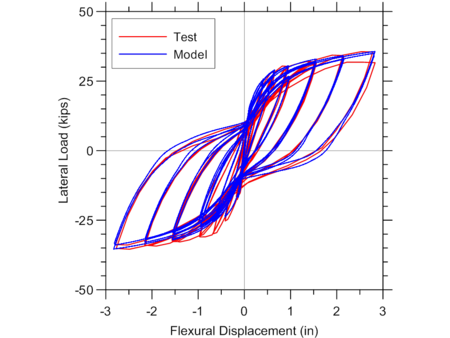
Figure E1.3 illustrates the sensitivity of analytical predictions obtained using the MVLEM to the optional gap closure parameter of the ConcreteCM model (-GapClose $gap, LINK), which allows consideration of different intensities of gradual gap closure in concrete (Figure E1.3a), as well as selection of the steel material model SteelMPF versus Steel02 (Figure E1.3b). It can be observed from Figure E1.3a that pinching characteristics of the response are slightly more pronounced when less gradual gap closure versus more gradual gap closure (i.e., gap=0 versus gap=1) is adopted. Figure E1.3b illustrates that the wall yield capacity as well as pinching characteristics of the behavior predicted by the MVLEM vary slightly when SteelMPF versus Steel02 is used.
For illustration purposes, additional response predictions obtained using the MVLEM model are presented in Figure E1.4 and Figure E1.5, where analytically-predicted strain histories at the outermost and central wall fibers, and concrete and steel strain-stress relationships at the outermost fiber are presented, respectively. Responses are obtained using MVLEM recorders Fiber_Strain, Fiber_Stress_Concrete, and Fiber_Stress_Steel.
Element SFI_MVLEM - Cyclic Shear-Flexure Interaction Model for RC Walls
Developed and Implemented by:
Kristijan Kolozvari, California State University, Fullerton
Kutay Orakcal, Bogazici University, Istanbul, Turkey
John Wallace, Univeristy of California, Los Angeles
The SFI_MVLEM command is used to construct a Shear-Flexure Interaction Multiple-Vertical-Line-Element Model (SFI-MVLEM, Kolozvari et al., 2014a, b), which captures interaction between axial/flexural and shear behavior of RC structural walls and columns under cyclic loading. The SFI_MVLEM element (Figure 1) incorporates 2-D RC panel behavior described by the Fixed-Strut-Angle-Model (nDMaterial FSAM; Ulugtekin, 2010; Orakcal et al., 2012), into a 2-D macroscopic fiber-based model (MVLEM). The interaction between axial and shear behavior is captured at each RC panel (macro-fiber) level, which further incorporates interaction between shear and flexural behavior at the SFI_MVLEM element level.
Source: /usr/local/cvs/OpenSees/SRC/element/SFI_MVLEM/
Input Format:
| Element SFI_MVLEM $eleTag $iNode $jNode $m $c -thick {Thicknesses} -width {Widths} -mat {Material_tags} |
| $eleTag | Unique element object tag |
| $iNode $jNode | End node tags |
| $m | Number of element macro-fibers |
| $c | Location of center of rotation with from the iNode, c = 0.4 (recommended) |
| {Thicknesses} | Array of m macro-fiber thicknesses |
| {Widths} | Array of m macro-fiber widths |
| {Material_tags} | Array of m macro-fiber nDMaterial1 tags |
1SFI_MVLEM element shall be used with nDMaterial FSAM, which is a 2-D plane-stress constitutive relationship representing reinforced concrete panel behavior.
Element Recorders:
The following recorders are available with the SFI_MVLEM element:
| globalForce | Element global forces |
| Curvature | Element curvature |
| ShearDef | Element shear deformation |
| RCPanel $fibTag $Response | Returns RC panel (macro-fiber) $Response for a $fibTag-th panel (1 ≤ fibTag ≤ m). For available $Response-s refer to nDMaterial FSAM (LINK). |
Examples:
Element SFI_MVLEM 1 1 2 5 0.4 -thick 6 6 6 6 6 -width 9 10 10 10 9 -mat 7 6 6 6 7
Recorder Element -file SFI_MVLEM_Fgl.out -time -ele 1 2 3 globalForce
Recorder Element -file SFI_MVLEM_panel_strain.out -time -ele 1 RCPanel 1 panel_strain
References:
1) Kolozvari K., Orakcal K., and Wallace J. W. (2015a). ”Modeling of Cyclic Shear-Flexure Interaction in Reinforced Concrete Structural Walls. I: Theory”, ASCE Journal of Structural Engineering, 141(5), 04014135 doi
2) Kolozvari K., Tran T., Orakcal K., and Wallace, J.W. (2015b). ”Modeling of Cyclic Shear-Flexure Interaction in Reinforced Concrete Structural Walls. II: Experimental Validation”, ASCE Journal of Structural Engineering, 141(5), 04014136 doi
3) Kolozvari K. (2013). “Analytical Modeling of Cyclic Shear-Flexure Interaction in Reinforced Concrete Structural Walls”, PhD Dissertation, University of California, Los Angeles.
Example 1. Simulation of Shear-Flexural Behavior of a Medium-Rise RC Wall Specimen under Cyclic Loading using the SFI-MVLEM Model
The behavior of RC wall specimen RW-A15-P10-S78 (Tran and Wallace, 2012) tested under constant axial load and cyclic lateral displacement history applied at the top of the wall is predicted using the SFI_MVLEM model. The input parameters and output results are presented in the following sections.
E1.1. Model Calibration
Basic properties of the specimen with model discretization are shown on Figure E1.1. Detailed information about the test specimen can be found in paper by Tran and Wallace (2012), whereas details of model calibration are provided by Kolozvari (2013) and Kolozvari et al. (2015b).
E1.2. Input Files
Input files (.tcl) used to build the wall model and perform displacement-controlled analysis can be found in Example 1. SFI_MVLEM.zip:
- SFI_MVLEM_SP4.tcl – model generation and definition of analysis parameters
- gravity.tcl – application of gravity load
- dispControl.tcl – application of lateral displacement history (run this file)
- LibAnalysisStaticParameters.tcl - definition of static analysis parameters
- LibGeneratePeaks.tcl - generation of displacement history
E1.3. Analysis Results
The following sub-section presents analytical results obtained for the test specimen described above, using the input files provided. The results include global wall responses (compared against experimental results), model element responses, and individual RC panel (macro-fiber) responses.
E1.3.1. Global Wall Responses
Analytical and experimental lateral load versus top total displacement responses and wall cracking patterns are presented on Figure E1.2, whereas lateral load versus flexural and shear deformations are shown on Figure E1.3. Total top displacement is obtained from the top node, shear force is recorded using globalForce element recorder, total shear displacement is obtained using shearDef element recorder and crack orientations are obtained using RCPanel and cracking_angles element recorders.
E1.3.2. Model Element Responses
Figure E1.4 plots lateral load versus total, flexural and shear displacement responses, as well as moment versus curvature relationship, obtained from the analysis for the bottom wall model element. Responses are recorded using globalForce, ShearDef, and Curvature element recorders.
E1.3.3. Reinforced Concrete Panel Responses
Various stress-strain responses for an individual boundary panel element (outermost macro-fiber) within the bottommost wall element are presented, including total (resultant) stress vs. strain relationships in the xy plane (Figure E1.5; element RCPanel recorders: panel_strain and panel_stress), stress-strain relationships along the two concrete struts (Figure E1.6; element RCPanel recorders: strain_stress_concrete1 and strain_stress_concrete2), and stress-strain relationship along horizontal and vertical steel reinforcement (Figure E1.7; element RCPanel recorders: strain_stress_steelX and strain_stress_steelY).
Example 2. Dynamic Analysis of a Coupled Wall-Frame System
This example illustrates application of the SFI_MVLEM wall model for nonlinear dynamic analysis. Analytical model of a coupled wall-frame building system was generated and analyzed under a single ground motion time-history. Brief description of the building characteristics and the analytical model are provided in the following sections.
E2.1. Building Description
Plan and elevation/section views of the considered building are shown in Figure E2.1. The building footprint is 140 ft × 60 ft, with 20 ft long spans. Analysis is conducted for shaking in the transverse direction only, where the lateral-force-resisting elements include two identical one-bay frames located at the building perimeter (axis 1 and 8, Figure E2.1a) and two identical walls located near the center of the building (axis 4 and 5, Figure E2.1a). Structural design is performed for a residential building (I=1.0, risk category I, design category D; ASCE 7-10 S11.5 and S11.6) for uniformly distributed dead load of 150 psf and live load of 40 psf (ASCE 7-10, Table 4-1), as well as the earthquake lateral loading obtained using Equivalent Lateral Force Procedure of ASCE 7-10 (S12.8). The frame was designed to resist 25% of the earthquake lateral load (Dual System, ASCE 7-10). Concrete compressive strength of f’c = 5,000 psi and reinforcing steel (both longitudinal and transversal reinforcement) with yield strength fy = 60,000 psi were used. Based on the structural design, cross-section dimensions of 12 in × 240 in (walls), 18 in × 32 in (beams; width × depth), and 28 in × 28 in (columns) were adopted. Cross-sections of structural elements with the reinforcement detailing are provided in Figure E2.2.
E2.2. Analytical Model Description
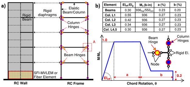
Due to building symmetry and applied direction of the ground motion, a two-dimensional model consisting of one frame and one wall (Figure E2.3) is used to simulate the building behavior. The gravity system is not included in the model (ASCE 7-10) and the assumption of a rigid diaphragm is implemented within each story level. Tributary mass is assigned at the element nodes at each story level at locations of axes of the vertical elements (i.e., wall and columns), whereas gravity load (dead and live) was assigned according to corresponding tributary areas as either nodal load at wall-element nodes of each story or uniformly distributed load along the beams of the frame.
As show on Figure E2.3, the RC wall is modeled using ten equal-length SFI_MVLEM elements along the wall height (i.e., two elements per story height). Wall discretization in horizontal direction was performed using six macro-fibers to represent the wall cross section, where two outer macro-fibers were used to represent the confined wall boundaries and the remaining four represent the unconfined wall web. Material models for steel and concrete are calibrated based on adopted material strengths to represent the behavior of confined and unconfined concrete and reinforcing steel.
RC frame elements (i.e., beams and columns) are modeled using elastic beam-column elements by assuming the location of plastic hinges at the faces of beam-column joints (Figure E2.3a), the behavior of which was simulated using zero-length elements at locations of hinges and the elasto-plastic moment-rotation hysteretic model (Modified Ibarra Krawinkler Deterioration Model; Lignos and Krawinkler, 2011), with modeling parameters adopted according to beam and column flexural capacities and the ASCE 41 backbone relationships (Figure E2.3b). The reduction of flexural stiffness after cracking was considered using stiffness modifiers for elastic portions of beam and column elements according to ASCE 41 (Table 6.5).
E2.3. Input Files
Input files (.tcl) used to build the model of a 5-story wall-frame system and perform gravity and dynamic analysis can be found in Example 2. SFI_MVLEM.zip:
- 5storyWF_SFI.tcl – model generation, definition of analysis parameters, gravity analysis
- Modal.tcl – modal analysis
- Dynamic.tcl – application of earthquake acceleration time-history (run this file)
- MCEScaledEQ1X.acc – earthquake acceleration time history file
- DisplayModel2D.tcl - display 2D model
- DisplayPlane.tcl - display plane
E2.4. Dynamic Analysis Results
Results obtained using analytical model of the building described in the previous section are presented, including modal properties of the structure, wall global (i.e., lateral deformations, drifts, shear force, moments) and local (i.e., vertical strains and rotations) responses. Responses of the structural elements comprising the RC frame are not considered.
E2.4.1. Dynamic Properties
First two building fundamental periods and mode shapes are presented in Figure E2.4.

E2.4.2. Time-history Responses
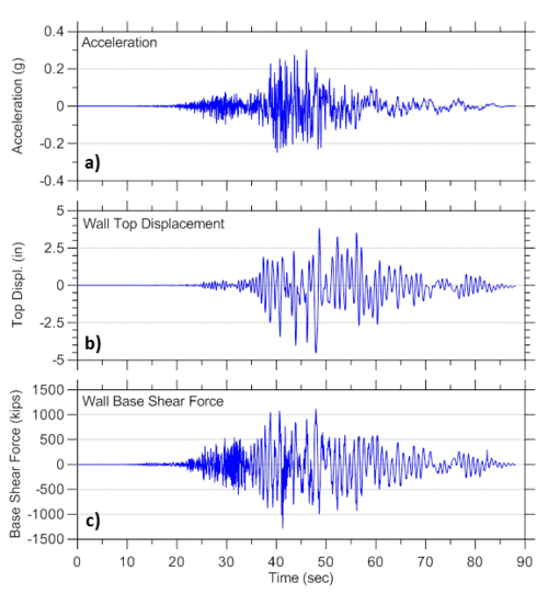
Time histories of ground motion acceleration, wall top nodal displacement, and wall base shear force (bottom wall node reaction) are presented in Figure 2.5; the responses are obtained using globalForce and Reactions node recorders.
E2.4.3. Maximum Global Responses over the Wall Height
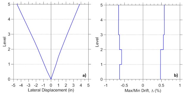
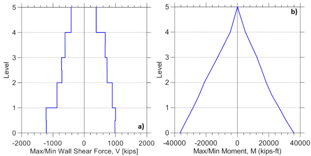
Maximum envelopes of wall lateral displacements and interstory drifts, and shear force and bending moment are presented in Figure E2.6 and Figure E2.7, respectively. Wall lateral displacements and drifts are obtained using corresponding node recorders, disp and drift, whereas shear force and bending moments over the wall height are recorded using element recorders globalForce.
E2.4.4. Bottom Wall Element Responses
Figure E2.8 plots the responses of the bottom wall element, including lateral load versus total, flexural and shear displacement, and moment versus curvature relationship obtained from the dynamic analysis. Note that wall element shear displacement and curvature time-histories are obtained using SFI_MVLEM element recorders ShearDef and Curvature, respectively, whereas shear force and bending moment are recorded using element recorder globalForce.
E2.4.5. Single RC Panel Responses
Analytically-predicted strain-stress responses of a single RC panel (macro-fiber) located at the left wall boundary of the bottom wall element are presented. Global panel stress-strain relationships presented on Figure E2.9 are obtained using element recorder RCPanel with commands panel_strain and panel_stress; the uniaxial behavior of concrete along the two concrete struts presented on Figure E2.10 are recorded using strain_stress_concrete1 and strain_stress_concrete2 commands; uniaxial stress-strain behavior of horizontal and vertical reinforcing steel presented on Figure E2.11 are obtained using strain_stress_steelX and strain_stress_steelY commands. Other panel responses described in Section 3 could be plotted in a similar manner.
Finally, vertical profiles of maximum vertical strains (Figure E2.12a) are obtained using element recorder with RCPanel and panel_strain recorder commands, whereas maximum wall rotations over the wall height (Figure E2.12b) are derived from element Curvature recorder. Similarly, the distribution of other wall responses could be plotted over the wall height (e.g., shear deformations, etc.).
uniaxialMaterial SteelMPF - Steel Material Model by Menegotto and Pinto (1973) extended by Filippou et al. (1983)
Developed and Implemented by:
Kristijan Kolozvari, California State University, Fullerton
Kutay Orakcal, Bogazici University, Istanbul, Turkey
John Wallace, Univeristy of California, Los Angeles
This command is used to construct a uniaxialMaterial SteelMPF, which represents the well-known uniaxial constitutive nonlinear hysteretic material model for steel proposed by Menegotto and Pinto (1973), and extended by Filippou et al. (1983) to include isotropic strain hardening effects. The relationship is in the form of curved transitions (Figure 1), each from a straight-line asymptote with slope E0 (modulus of elasticity) to another straight-line asymptote with slope E1 = bE0 (yield modulus) where b is the strain hardening ratio. The curvature of the transition curve between the two asymptotes is governed by a cyclic curvature parameter R, which permits the Bauschinger effect to be represented, and is dependent on the absolute strain difference between the current asymptote intersection point and the previous maximum or minimum strain reversal point depending on whether the current strain is increasing or decreasing, respectively. The strain and stress pairs (εr,σr) and (ε0,σ0) shown on Figure 1 are updated after each strain reversal.
Source: /usr/local/cvs/OpenSees/SRC/material/uniaxial/
Input Format:
| uniaxialMaterial SteelMPF $mattag $fyp $fyn $E0 $bp $bn $R0 $a1 $a2 <$a3 $a4> |
| $mattag | Unique uniaxialMaterial tag |
| $fyp | Yield strength in tension (positive loading direction) |
| $fyn | Yield strength in compression (negative loading direction) |
| $E0 | Initial tangent modulus |
| $bp | Strain hardening ratio in tension (positive loading direction) |
| $bn | Strain hardening ratio in compression (negative loading direction) |
| $R0 | Initial value of the curvature parameter R (R0 = 20 recommended) |
| $a1 | Curvature degradation parameter (a1 = 18.5 recommended) |
| $a2 | Curvature degradation parameter (a2 = 0.15 or 0.0015 recommended) |
| $a3 | Isotropic hardening parameter (optional, default = 0.01) |
| $a4 | Isotropic hardening parameter (optional, default = 7.0) |
Example:
uniaxialMaterial SteelMPF 1 60 60 29000 0.02 0.02 20.0 18.5 0.15
Discussion:
Although the Menegotto-Pinto model is already available in OpenSees (e.g., Steel02), the formulation of SteelMPF introduces several distinctive features compared to existing models. For example, the model allows definition of different yield stress values and strain hardening ratios for tension and compression, and it considers degradation of cyclic curvature parameter R for strain reversals in both pre- and post- yielding regions, which could produce more accurate predictions of yield capacity for some RC wall specimens (see LINK Example 1), whereas Steel02 considers the degradation in post-yielding region only. Strain-stress relationships obtained using SteelMPF and Steel02 are compared in Figure 2 for a strain history that includes strain reversals at strain values equal to one-half of the yield strain (e.i., <math>\epsilon</math>r = ±0.001 = <math>\epsilon</math>y/2). The model also allows calibration of isotropic hardening parameters through optional input variables a3 and a4, and uses default values of a3 = 0.01 and a4 = 7.0 as calibrated by Filippou et al. (1983) based on test results. To disregard isotropic strain hardening behavior in SteelMPF, parameter a3 needs to be assigned a zero value (a3 = 0.0).
References:
1) Filippou F.C., Popov, E.P., and Bertero, V.V. (1983). "Effects of Bond Deterioration on Hysteretic Behavior of Reinforced Concrete Joints". Report EERC 83-19, Earthquake Engineering Research Center, University of California, Berkeley.
2) Menegotto, M., and Pinto, P.E. (1973). Method of analysis of cyclically loaded RC plane frames including changes in geometry and non-elastic behavior of elements under normal force and bending. Preliminary Report IABSE, vol 13.
uniaxialMaterial ConcreteCM - Complete Concrete Model by Chang and Mander (1994)
Developed and Implemented by:
Kristijan Kolozvari, California State University, Fullerton
Kutay Orakcal, Bogazici University, Istanbul, Turkey
John Wallace, Univeristy of California, Los Angeles
This command is used to construct a uniaxialMaterial ConcreteCM, which is a uniaxial hysteretic constitutive model for concrete developed by Chang and Mander (1994). This model is a refined, rule-based, generalized, and non-dimensional constitutive model that allows calibration of the monotonic and hysteretic material modeling parameters, and can simulate the hysteretic behavior of confined and unconfined, ordinary and high-strength concrete, in both cyclic compression and tension (Figure 1). The model addresses important behavioral features, such as continuous hysteretic behavior under cyclic compression and tension, progressive stiffness degradation associated with smooth unloading and reloading curves at increasing strain values, and gradual crack closure effects. Details of the model are available in the report by Chang and Mander (1994).
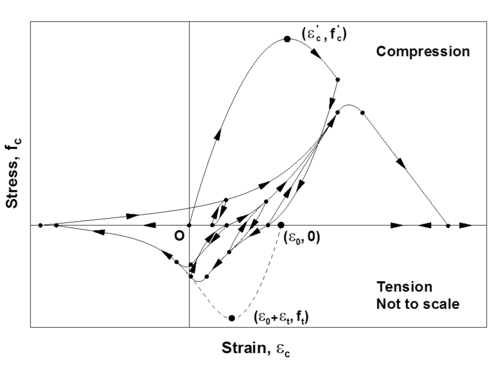
The Chang and Mander (1994) model successfully generates continuous hysteretic stress-strain relationships with slope continuity for confined and unconfined concrete in both compression and tension. The compression envelope curve of the model is defined by the initial tangent slope, (Ec), the peak coordinate (<math>\epsilon</math>'c, f'c), a parameter (rc) from Tsai’s (1988) equation defining the shape of the envelope curve, and a parameter (<math>\epsilon</math>-cr) to define normalized (with respect to <math>\epsilon</math>'c) strain where the envelope curve starts following a straight line, until zero compressive stress is reached at the spalling strain, <math>\epsilon</math>sp. These parameters can be controlled based on specific experimental results for a refined calibration of the compression envelope (Figure 2). Chang and Mander (1994) proposed empirical relationships for parameters Ec, <math>\epsilon</math>'c, and rc for unconfined concrete with compressive strength f'c, based on review of previous research. Parameters f'c, <math>\epsilon</math>'c, Ec, rc, and <math>\epsilon</math>-cr can also be calibrated to represent the stress-strain behavior of confined concrete in compression, to follow the constitutive relationships for confined concrete proposed by Mander et al (1988) or similar.
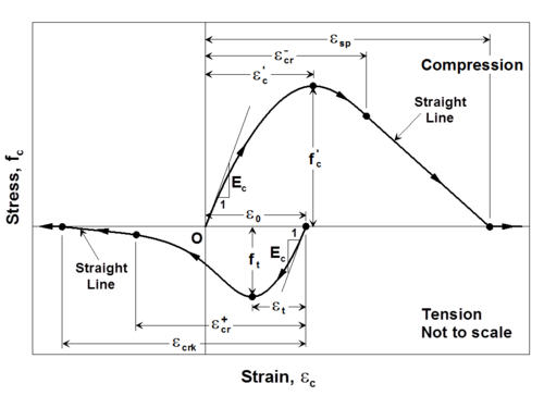
The shape of the tension envelope curve in the model is the same as that of the compression envelope; however, the tension envelope curve is shifted to a new origin that is based on the unloading strain from the compression envelope (Figure 2). As well, the strain ductility experienced previously on the compression envelope is also reflected on the tension envelope. The parameters associated with the tension envelope curve include the tensile strength of concrete (ft), the monotonic strain at tensile strength (<math>\epsilon</math>t), a parameter (rt) from Tsai’s (1988) equation defining the shape of the tension envelope curve, and a parameter (<math>\epsilon</math>+cr) to define normalized (with respect to <math>\epsilon</math>t) strain where the tension envelope curve starts following a straight line, until zero tensile stress is reached at a strain of <math>\epsilon</math>crk. These parameters can also be controlled and calibrated based on specific experimental results or empirical relations proposed by other researchers (e.g., Belarbi and Hsu, 1994) to model the behavior of concrete in tension and the tension stiffening phenomenon. Concrete experiencing tension stiffening can be considered not to crack completely; that is, a large value for parameter <math>\epsilon</math>+cr (e.g., 10000) can be defined.
Source: /usr/local/cvs/OpenSees/SRC/material/uniaxial/
Input Format:
| uniaxialMaterial ConcreteCM $mattag $fpcc $epcc $Ec $rc $xcrn $ft $et $rt $xcrp <-GapClose $gap> |
| $mattag | Unique uniaxialMaterial tag |
| $fpcc | Compressive strength (f'c) |
| $epcc | Strain at compressive strength (<math>\epsilon</math>'c) |
| $Ec | Initial tangent modulus (Ec) |
| $rc | Shape parameter in Tsai’s equation defined for compression (rc) |
| $xcrn | Non-dimensional critical strain on compression envelope (<math>\epsilon</math>-cr, where the envelope curve starts following a straight line) |
| $ft | Tensile strength (ft) |
| $rt | Shape parameter in Tsai’s equation defined for tension (rt) |
| $xcrp | Non-dimensional critical strain on tension envelope (<math>\epsilon</math>+cr, where the envelope curve starts following a straight line – large value [e.g., 10000] recommended when tension stiffening is considered) |
| <-GapClose $gap> | gap = 0, less gradual gap closure (default); gap = 1, more gradual gap closure |
Example:
uniaxialMaterial ConcreteCM 1 -6.2 -0.0021 4500 7 1.035 0.30 0.00008 1.2 10000
Example of hysteretic stress–strain history generated by the model code is illustrated in Figure 3.
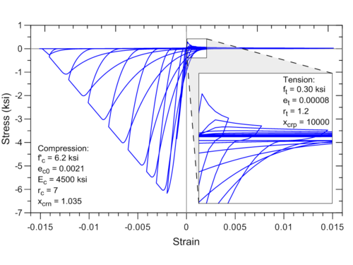
Discussion:
An optional input parameter gap is introduced in the ConcreteCM model implemented in OpenSees for providing the users with the opportunity to control the intensity of gap closure in the stress-strain behavior of concrete, which in-turn influences the level of pinching in the lateral load-displacement behavior of a RC wall. The original Chang and Mander (1994) model adopts a non-zero tangent stiffness at zero stress level upon unloading from the tension envelope, which is represented by gap = 1 in ConcreteCM. Using gap = 0 (default) produces less gradual gap closure, since it assumes zero tangent stiffness at zero stress level upon unloading from the tension envelope, and is suitable for most analyses. Figure 4 illustrates the effect of plastic stiffness upon unloading from tension envelope (E+pl) on crack closure, i.e. use of more gradual (gap = 1) or less gradual (gap = 0) gap closure.
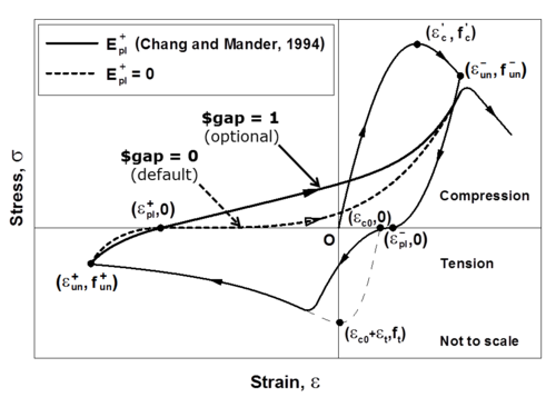
Constitutive stress-strain concrete behavior is also implemented in OpenSees in uniaxialMaterial Cocnrete07. However, ConcreteCM incorporates sophisticated unloading/reloading rules defined originally by Chang and Mander (1994), as opposed to Concrete07 that adopts simplified hysteretic rules. Comparison between stress-strain response predicted using ConcreteCM and Concrete07 is shown in Figure 5.
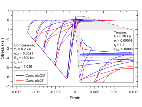
References:
1) Belarbi H. and Hsu T.C.C. (1994). “Constitutive Laws of Concrete in Tension and Reinforcing Bars Stiffened by Concrete”, ACI Structural Journal, V. 91, No. 4, pp. 465-474.
2) Chang, G.A. and Mander, J.B. (1994), “Seismic Energy Based Fatigue Damage Analysis of Bridge Columns: Part I – Evaluation of Seismic Capacity”, NCEER Technical Report No. NCEER-94-0006, State University of New York, Buffalo.
3) Mander J.B., Priestley M.J.N., and Park R. (1988). “Theoretical Stress-Strain Model for Confined Concrete”, ASCE Journal of Structural Engineering, V. 114, No. 8, pp. 1804-1826.
4) Orakcal K.(2004), "Nonlinear Modeling and Analysis of Slender Reinforced Concrete Walls", PhD Dissertation, Department of Civil and Environmental Engineering, University of California, Los Angeles.
NDMaterial FSAM - 2D RC Panel Constitutive Behavior
Developed and Implemented by:
Kristijan Kolozvari, California State University, Fullerton
Kutay Orakcal, Bogazici University, Istanbul, Turkey
Leonardo Massone, University of Chile, Santiago
John Wallace, Univeristy of California, Los Angeles
This command is used to construct a nDMaterial FSAM (Fixed-Strut-Angle-Model, Figure 1), which is a plane-stress constitutive model for simulating the behavior of RC panel elements under generalized, in-plane, reversed-cyclic loading conditions (Ulugtekin, 2010; Orakcal et al., 2012). In the FSAM constitutive model, the strain fields acting on concrete and reinforcing steel components of a RC panel are assumed to be equal to each other, implying perfect bond assumption between concrete and reinforcing steel bars. While the reinforcing steel bars develop uniaxial stresses under strains in their longitudinal direction, the behavior of concrete is defined using stress–strain relationships in biaxial directions, the orientation of which is governed by the state of cracking in concrete. Although the concrete stress–strain relationship used in the FSAM is fundamentally uniaxial in nature, it also incorporates biaxial softening effects including compression softening and biaxial damage. For transfer of shear stresses across the cracks, a friction-based elasto-plastic shear aggregate interlock model is adopted, together with a linear elastic model for representing dowel action on the reinforcing steel bars (Kolozvari, 2013).
Source: /usr/local/cvs/OpenSees/SRC/material/nD/reinforcedConcretePlaneStress/
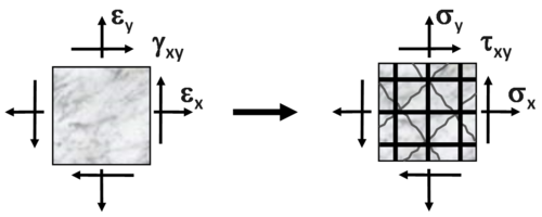
Input Format:
| nDMaterial FSAM $mattag $rho $sX $sY $conc $rouX $rouY $nu $alfadow |
| $mattag | Unique nDMaterial tag |
| $rho | Material density |
| $sX | Tag of uniaxialMaterial simulating horizontal (x) reinforcement |
| $sY | Tag of uniaxialMaterial simulating vertical (y) reinforcement |
| $conc | Tag of uniaxialMaterial1 simulating concrete |
| $rouX | Reinforcing ratio in horizontal (x) direction (rouX = As,x/Agross,x) |
| $rouY | Reinforcing ratio in vertical (y) direction (rouY = As,y/Agross,y) |
| $nu | Concrete friction coefficient (0.0 < nu < 1.5) |
| $alfadow | Stiffness coefficient of reinforcement dowel action (0.0 < alfadow < 0.05) |
1nDMaterial FSAM shall be used with uniaxialMaterial ConcreteCM
Recommended values for parameter of a shear resisting mechanism (nu and alfadow, Figure 2) are provided above. Details about the sensitivity of analytical predictions using SFI_MVLEM to changes in these parameters are presented by Kolozvari (2013).
Material Recorders:
The following output is available from the FSAM RC panel model:
| panel_strain | Strains εx, εy, γxy (Figure 4) |
| panel_stress | Resulting panel stresses σx, σy, τxy (concrete and steel, Figure 1) |
| panel_stress_concrete | Resulting panel concrete stresses σxc, σyc, τxyc (Figure 2b) |
| panel_stress_steel | Resulting panel steel stresses σxs, σys, τxys (Figure 2d) |
| strain_stress_steelX | Uniaxial strain and stress of horizontal reinforcement εx, σxxs |
| strain_stress_steelY | Uniaxial strain and stress of vertical reinforcement εy, σyys |
| strain_stress_concrete1 | Uniaxial strain and stress of concrete strut 1 εc1, σc1 |
| strain_stress_concrete2 | Uniaxial strain and stress of concrete strut 2 εc2, σc2 |
| strain_stress_interlock1 | Shear strain and stress in concrete along crack 1 εcr1, τcr1 (Figure 2c) |
| strain_stress_interlock2 | Shear strain and stress in concrete along crack 2 εcr2, τcr2 (Figure 2c) |
| cracking_angles | Orientation of concrete cracks |
Note that recorders for a RC panel (marco-fiber) are invoked as SFI_MVLEM element recorders using command RCPanel and one of the desired commands listed above. Currently, it is possible to output values only for one macro-fiber within one or multiple elements.
Example:
nDMaterial FSAM 1 0.0 1 2 4 0.0073 0.0606 0.1 0.01
Recorder Element -file MVLEM_panel_strain.out -time -ele 1 RCPanel 1 panel_strain
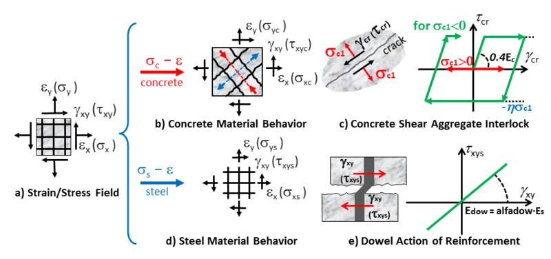
References:
1) Kolozvari K. (2013). “Analytical Modeling of Cyclic Shear-Flexure Interaction in Reinforced Concrete Structural Walls”, PhD Dissertation, University of California, Los Angeles.
2) Orakcal K., Massone L.M., and Ulugtekin D. (2012). “Constitutive Modeling of Reinforced Concrete Panel Behavior under Cyclic Loading”, Proceedings, 15th World Conference on Earthquake Engineering, Lisbon, Portugal.
3) Ulugtekin D. (2010). “Analytical Modeling of Reinforced Concrete Panel Elements under Reversed Cyclic Loadings”, M.S. Thesis, Bogazici University, Istanbul, Turkey.