Reinforced Concrete Frame Gravity Analysis

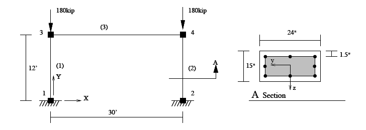
This example subjects the reinforced concrete portal frame, shown below, to gravity loads.

Here is the file: RCFrameGravity.tcl

Model

A nonlinear model of the portal frame is created, The model consists of four nodes, two force beam column elements to model the columns and an elastic beam (3) to model the beam. For the column elements, a section identical to the one used in Moment Curvature Example, is created using steel and concrete fibers. The bottom two nodes are fixed and a single load pattern with a Linear time series is created. Two vertical loads acting at node 3 and 4 are added to this pattern.

# Create ModelBuilder (with two-dimensions and 3 DOF/node)
model basic -ndm 2 -ndf 3

# Create nodes
# ------------

# Set parameters for overall model geometry
set width    360
set height   144

# Create nodes
#    tag        X       Y 
node  1       0.0     0.0 
node  2    $width     0.0 
node  3       0.0 $height
node  4    $width $height


# Fix supports at base of columns
#    tag   DX   DY   RZ
fix   1     1    1    1
fix   2     1    1    1

# Define materials for nonlinear columns# ------------------------------------------
# CONCRETE                  tag  f'c    ec0    f'cu      ecu
# Core concrete (confined)
uniaxialMaterial Concrete01  1  -6.0  -0.004   -5.0     -0.014

# Cover concrete (unconfined)
uniaxialMaterial Concrete01  2  -5.0  -0.002    0.0     -0.006

# STEEL
# Reinforcing steel 
#                        tag  fy  E0    b
uniaxialMaterial Steel01  3  60.0 3000.0 0.01

# Define cross-section for nonlinear columns
# ------------------------------------------

# set some paramaters
set colWidth 15
set colDepth 24 

set cover  1.5

set As    0.60;     # area of no. 7 bars

# some variables derived from the parameters
set y1 [expr $colDepth/2.0]
set z1 [expr $colWidth/2.0]

section Fiber 1 {

    # Create the concrete core fibers
    patch rect 1 10 1 [expr $cover-$y1] [expr $cover-$z1] [expr $y1-$cover] [expr $z1-$cover]

    # Create the concrete cover fibers (top, bottom, left, right)
    patch rect 2 10 1  [expr -$y1] [expr $z1-$cover] $y1 $z1
    patch rect 2 10 1  [expr -$y1] [expr -$z1] $y1 [expr $cover-$z1]
    patch rect 2  2 1  [expr -$y1] [expr $cover-$z1] [expr $cover-$y1] [expr $z1-$cover]
    patch rect 2  2 1  [expr $y1-$cover] [expr $cover-$z1] $y1 [expr $z1-$cover]

    # Create the reinforcing fibers (left, middle, right)
    layer straight 3 3 $As [expr $y1-$cover] [expr $z1-$cover] [expr $y1-$cover] [expr $cover-$z1]
    layer straight 3 2 $As 0.0 [expr $z1-$cover] 0.0 [expr $cover-$z1]
    layer straight 3 3 $As [expr $cover-$y1] [expr $z1-$cover] [expr $cover-$y1] [expr $cover-$z1]

}    

# Define column elements
# ----------------------

# Geometry of column elements
#                tag 
geomTransf Linear 1  

# Number of integration points along length of element
set np 5

set eleType forceBeamColumn; # forceBeamColumn od dispBeamColumn will work

# Create the coulumns using Beam-column elements
#                 tag ndI ndJ nsecs secID transfTag
element $eleType  1   1   3   $np    1       1 
element $eleType  2   2   4   $np    1       1 

# Define beam elment
# -----------------------------

# Geometry of column elements
#                tag 
geomTransf Linear 2  

# Create the beam element
#                          tag ndI ndJ     A       E    Iz   transfTag
element elasticBeamColumn   3   3   4    360    4030  8640    2


# Define gravity loads
# --------------------

# Set a parameter for the axial load
set P 180;                # 10% of axial capacity of columns

# Create a Plain load pattern with a Linear TimeSeries
timeSeries Linear 1
pattern Plain 1 1 {

        # Create nodal loads at nodes 3 & 4
	#    nd    FX          FY  MZ 
	load  3   0.0  [expr -$P] 0.0
	load  4   0.0  [expr -$P] 0.0
}

Analysis

This model contains material non-linearities, so a nonlinear solution algorithm of type Newton is used. The solution algorithm requires a convergence test to determine if convergence at each trial step has been achieved. For this example we will use the norm of the displacement increment vector. Also for this nonlinear example, we will apply the loads gradually in 0.1 incremental steps using a LoadControl strategy until the full load is applied. The eauations will be stored and solved using a banded general storae scheme and solver. To minimise the band of this solver, a reverse Cuthill-McKee (RCM) numbering scheme will be used. The constrains are enforced using the Plain constraint handler.

Once the static analysis is created, 10 analysis steps are needed to bring the full gravity load to bear on the model. (10 * 0.1 = 1.0)

# Create the system of equation, a sparse solver with partial pivoting
system BandGeneral

# Create the constraint handler, the transformation method
constraints Transformation

# Create the DOF numberer, the reverse Cuthill-McKee algorithm
numberer RCM

# Create the convergence test, the norm of the residual with a tolerance of 
# 1e-12 and a max number of iterations of 10
test NormDispIncr 1.0e-12  10 3

# Create the solution algorithm, a Newton-Raphson algorithm
algorithm Newton

# Create the integration scheme, the LoadControl scheme using steps of 0.1 
integrator LoadControl 0.1

# Create the analysis object
analysis Static

# Perform the analysis
analyze 10

Output

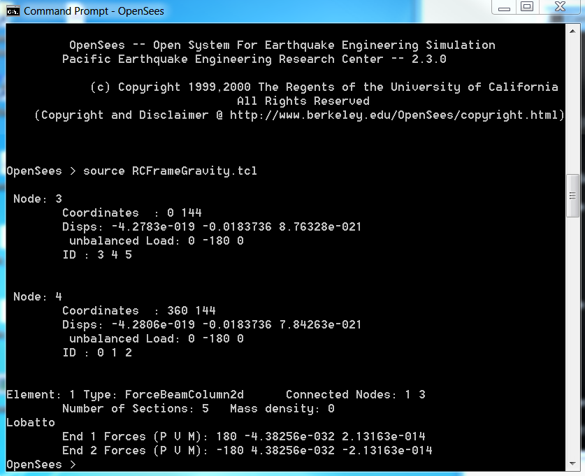
For output, we will look at the displacements at nodes 3 and 4 and the state of element 1.

# Print out the state of nodes 3 and 4
print node 3 4

# Print out the state of element 1
print ele 1

Running the Script

When the script is run the following will appear.