Effective Stress Site Response Analysis of a Layered Soil Column
Example prepared by: Christopher McGann and Pedro Arduino, University of Washington
Return to OpenSees Examples Page
This article describes the OpenSees implementation of an effective stress site response analysis of a layered deposit of cohesionless soil underlain by an elastic half-space. A single column of soil is modeled in 2D (with periodic boundary conditions to emulate a 1D analysis) and is subject to an earthquake excitation. Nine node quadrilateral elements with both displacement and pore pressure degrees of freedom enable the model to track changes in pore pressure and effective stress during the earthquake excitation. A Lysmer-Kuhlemeyer (1969) dashpot is utilized to account for the finite rigidity of the underlying elastic medium.
This article also briefly introduces the user to the pre- and post-process visualization tool GiD. Specifically, the means to generate GiD-compatible results from the data returned by the OpenSees recorders are provided and discussed. GiD is a powerful tool for visualizing data and generating meshes, among other things. It is especially helpful when working with 2D and 3D problems in OpenSees. The GiD tool can be downloaded from http://gid.cimne.upc.es/download.
Note: Most of the details of this analysis are identical to those in the Total Stress Site Response Analysis of a Layered Soil Column example posted in the Practical Examples area of this manual. This article will emphasize the attributes which are particular to the effective stress analysis. The user is referred to the total stress example for further information on details which may be omitted or quickly explained here.
Provided with this article are several files. Files which are required for the analysis are indicated. The files include:
- The example input file, freeFieldEffective.tcl (required for analysis)
- The velocity time history of the selected earthquake record, velocityHistory.out (required for analysis)
- A GiD post-process mesh file, freeFieldEffective.flavia.msh (generated automatically by running freeFieldEffective.tcl)
- A Matlab script, flaviaWriter.m, which can be used to reformat the recorded displacement, pore pressure, and stress data into a file which can be read by GiD for post-process visulization. Non-Matlab users may find the process represented by this file useful in creating an alternative means for accomplishing this reformatting.
- The post-process results file, freeFieldEffective.flavia.res, which is generated through the use of the flaviaWriter.m script. This file, combined with the file freeFieldEffective.flavia.msh, allows the user to visualize the results of the site response analysis using GiD.
All of the files mentioned above can be downloaded by clicking here.
To run this example, the user must download the input file, freeFieldEffective.tcl, and the velocity time history file, velocityHistory.out, and place them in a single directory. Once this has been done, the user can then run the analysis. The additional files described above are not essential to the analysis. They are provided to demonstrate how to use the GiD tool to visualize results from this type of analysis.
For further information into a site response analysis using OpenSees, the user is referred to the previously-mentioned total stress site response analysis example and/or the large set of examples developed at the University of California at San Diego available at http://cyclic.ucsd.edu/opensees. These examples utilize a wide variety of element and material formulations, as well as different boundary and loading conditions than those used in this example.
Model Description
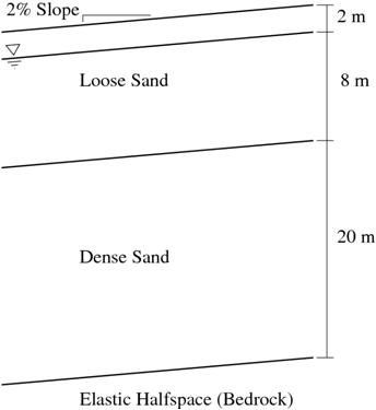
The site response analysis discussed in this article is for a soil profile consisting of a 10 m thick layer of loose sand (Dr = 40%) above a 20 m thick layer of more dense sand (Dr = 75%). The profile is assumed to be on an infinite slope with a 2% grade. A schematic representation of the analyzed soil profile is shown in Fig. 1. The entire soil profile is underlain by an elastic half-space which represents the finite rigidity of an underlying medium such as bedrock. The groundwater table is located at a depth of 2 m, therefore, saturated unit weights are used for the soil below this point and effective stress analysis is considered through the use of nine-node quadrilateral elements which are able to simulate fluid-solid coupling.
Mesh Geometry
The general layout of the model is similar to that discussed in the previously-posted total stress site response analysis example, however, the elements have nine nodes instead of four. A single nine-node element is shown in Fig. 2 to demonstrate the layout of the nodes and the order of element connectivity. The corner nodes (shown in blue in Fig. 2) have three degrees of freedom, two translational and one pore pressure, and the interior nodes (red in Fig. 2) have only two translational degrees of freedom.
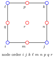
The implementation of the nine node quadrilateral element requires that the two types of nodes, and their corresponding fixities, be created in an appropriate domain. The pore pressure nodes their fixities must be preceded by the command
model BasicBuilder -ndm 2 -ndf 3,
indicating that the domain has 2 dimensions and 3 degrees of freedom. The interior nodes and corresponding fixities must be preceded by the command
model BasicBuilder -ndm 2 -ndf 2,
indicating that the domain has 2 dimensions and 2 degrees of freedom. The node and fixity definitions are the only major aspects of the model for which care must be taken with respect to the domain, however, since the load is applied to a corner node during the dynamic analysis, the correct domain must be redefined prior to the definition of the loading object.
The example analysis provided in the file freeFieldEffective.tcl is set-up in a manner such that the user need only define the geometry of the soil profile and groundwater table (Note: if the ground water table is not located at the surface, an additional soil layer must be included to differentiate the dry or moist soil above the gwt from the saturated soil below the gwt). The nodes are generated automatically based on the input geometry information. The input file is also set up such that different vertical element sizes can be used within each soil layer.
Boundary Conditions
The appropriate boundary conditions are also automatically generated based on the input geometry. The nodes at the base of the soil column are fixed against vertical translation and the pore pressure nodes above the groundwater table are fixed in the pore pressure dof (representing an open drainage condition). Periodic boundary conditions are assumed for the purposes of mimicking a 1D analysis. This is done though the use of the equalDOF command. For the periodic boundary condition, each of the nodes which share the same vertical location are given equal translational degrees of freedom. Note: The pore pressure degrees of freedom for corner nodes at a particular vertical location should not be linked using the equalDOF command. Through the creation of this example, it was found that this can cause problems in the analysis.
Material and Element Definitions
The soil constitutive behavior is modeled using the PressureDependMultiYield02 nDMaterial object. Since no attempt was made to model an actual soil deposit, the material parameters are based upon the recommended table of parameters available on the PressureDependMultiYield02 page for the appropriate relative densities.
Note: The mass density input values for the material objects should be total mass densities, i.e. above the groundwater table, the mass density should reflect dry or moist conditions, and below the groundwater table, the mass density should be the saturated value. For elements with free pore pressure degrees of freedom (those below the water table), the 9_4_QuadUP element computes the effective mass density using the input value from the material object and the fluid mass density specified during the element generation.
Included with the material definitions for each soil layer are additional parameters which are used by the 9_4_QuadUP element. These include the element thickness, the horizontal and vertical body forces on the element, the undrained bulk modulus, and the horizontal and vertical permeabilities. The example is set-up such that these values can vary from layer to layer. The creators of the 9_4_QuadUP element recommend an undrained bulk modulus which is equal to the bulk modulus of the fluid (2.2e6 kPa for water) divided by the porosity of the soil layer. For the layer above the groundwater table, a small value (5e-6 kPa) is used as the undrained bulk modulus.
Note: Gravity must be incorporated into an analysis using the 9_4_QuadUP element in a manner which differs from that used for the standard four node quad element. With the four node quad element, gravity is typically considered through the use of body forces which represent the unit weight of the soil. In the case of the nine node quad element, the body forces should not be the unit weights, instead they should have magnitudes equal to the components of gravity only, i.e. for an analysis of level ground using SI units, the vertical body force should be -9.81 and the horizontal body force should be zero. The infinite slope conditions of this example are modeled by using horizontal and vertical gravity components computed from the angle of the sloping ground as the body forces acting on the elements.
The 9_4_QuadUP elements are created automatically based on the input soil geometry and the material definitions. The 9_4_QuadUP element should be defined in the following manner:
element 9_4_QuadUP eleID nodei nodej nodek nodel nodem noden nodep nodeq noder thickness matID uBulk fMass hPerm vPerm hBody vBody
where uBulk is the undrained bulk modulus, fMass is the fluid mass density, hPerm and vPerm are the horizontal and vertical permeabilites, and hBody and vBody are the horizontal and vertical body forces. The nodal connectivity pattern matches that shown in Fig. 2. In this example, the fluid is water, therefore, the fluid mass density for each layer is set to 1.0 Mg/m^3.
The permeabilities for all of the elements are initially set to 1.0 m/s to ensure that hydrostatic conditions exist after the application of gravity in the model. If the permeability of a particular layer is too low, it may take many gravity analysis steps in order to reach hydrostatic pressure conditions. Prior to the application of the ground motion, the permeabilities of each soil layer are updated using the updateParameter command to their respective assigned values so pore pressure generation during the horizontal excitation is captured appropriately. The usage of the updateParameter command seems to differ from that documented here. Parameter tags must be defined for each permeability parameter (horizontal and vertical) for each element. Then these tags can be used to update the corresponding parameters.
An example of the parameter update process for two elements is provided here. To set the parameter tags:
#          tag             eleTag  parameterType
parameter  10001  element  1       vPerm
parameter  10002  element  1       hPerm
parameter  10003  element  2       vPerm
parameter  10004  element  2       hPerm
To update the permeability parameters:
#                tag    parameterValue
updateParameter  10001  1.0e-4
updateParameter  10002  1.0e-4
updateParameter  10003  1.0e-5
updateParameter  10004  1.0e-5
It seems to help to make the parameter tags different from any of the other tags used in the model (e.g. material, element tags), hence the numbers in this example start at 10001 and increase incrementally. As might be expected, the parameter tags must be defined before the parameters can be updated. The example input file included with this article is set up to automatically generate the parameter tags and update the permeability parameters.
The Lysmer-Kuhlemeyer (1969) dashpot nodes, material, and element are defined as described in the total stress site response analysis example using a bedrock shear wave velocity of 700 m/s and a bedrock mass density of 2.5 Mg/m^3.
Recorders and Analysis
The analysis consists of a gravity stage followed by a dynamic excitation stage. The recorders are separated in to two groups based on the analysis stages. The information recorded by the gravity recorders is useful to confirm that the model has been generated properly and that the appropriate conditions exist prior to the application of the horizontal excitation. A good place to start when working with a new model is the gravity phase. If the model doesn't converge or gives incorrect results under gravity loads, then it can never be expected to work properly in the remainder of the analysis.
The main details of the analysis phases are discussed in the total stress site response analysis example, however, there are several differences which will be discussed here. Due to the way in which this model is constrained, it seems that use of the penalty method works better than the transformation constraints used in the total stress example. The penalty factors specified in the example may need to be adjusted if changes are made to the geometry or parameters. The analysis seemed to run more smoothly using the Krylov-Newton algorithm as opposed to the standard Newton algorithm, however, the user is encouraged to experiment with different algorithms for their analyses. As previously noted above, the domain must be redefined to include three degrees of freedom prior to the definition of the loading object since the node at which the load is applied has three degrees of freedom.
Analysis Results
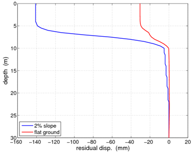
The fluid-solid coupling modeled by the 9_4_QuadUP element allows for the simulations of events such as liquefaction and lateral spreading. To demonstrate these situations, two distinct analyses were performed using the same soil profile. One analysis considers the 2% slope shown in Fig. 1 (and represented in the provided input file), and the other analysis considers level ground conditions. The flat ground case was simulated by setting the variable grade located in the material definition section of the input file to zero. In both cases, a portion of the loose sand layer becomes liquefied during the application of the ground motion. This fact is demonstrated in the included figures.
Fig. 3 shows the residual displacement profiles for the two conditions after the conclusion of the ground motion. As shown, there horizontal displacement of the upper portion of the soil column relative to the column base differs based upon the slope of the ground. With a 2% grade, approximately four times more relative displacement occurs, indicative of liquefaction-induced lateral spreading.
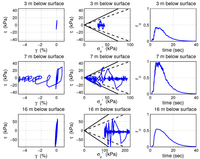
Figs. 4 and 5 summarize the soil behavior at depths of 3 m (above the liquefied zone), 7 m (in the middle of the liquefied zone), and 16 m (below the liquefied zone) for the level ground and sloping ground cases, respectively. These figures show the shear stress-strain behavior, the stress paths plotted on axes of shear stress vs. vertical effective stress, and the pore pressure ratios (computed as the ratio of excess pore pressure to initial effective vertical stress) as they vary with time. Included in the stress path plots are the failure and phase transformation surfaces for each respective location.
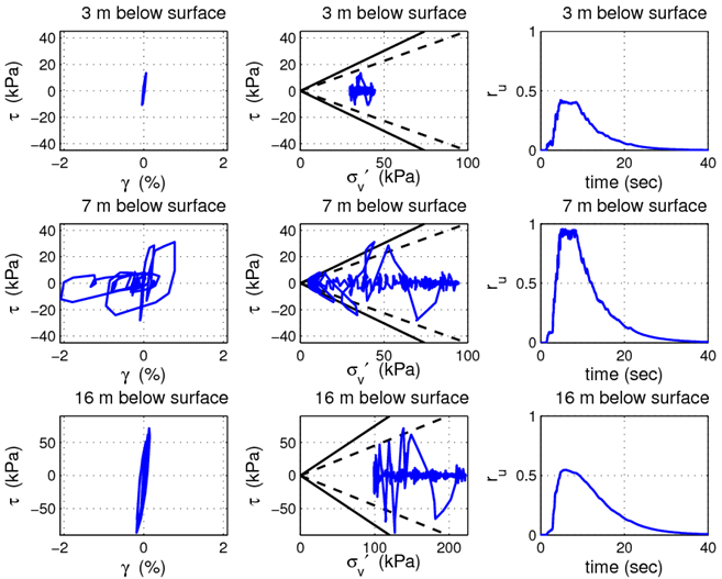
For both ground conditions, the results presented in Figs. 4 and 5 at a depth of 7 m are indicative of liquefaction. The pore pressure ratios both approach 1.0 (they never seem to quite get there in any of the simulations performed, there is likely som sort of tolerance in the elements) over a portion of the shaking, then become reduced with continued shaking. The stress path plots correspond, showing that the vertical effective stresses are reduced down towards zero as the soil liquefies, then strength is gained as the pore pressures dissipate with further shaking. The effects of the slope can be observed in Fig. 5, with the oscillations on the stress path plot being centered about a point which is not the zero shear stress axis.
The user can confirm the correct implementation of their downloaded version of this example by generating similar plots and comparing them to those included here. When generating the displacement profile plot, be sure to subtract the displacement of the base of the soil column from the values in order to create a plot which is the equivalent of that shown in Fig. 3.
GiD Visualization
As previously discussed, several files have been included in this article for the purpose of visualizing results in the pre- and post-processing tool GiD. The files related to this purpose are available for download here. The files are:
- freeFieldEffective.flavia.msh
- freeFieldEffective.flavia.res
- flaviaWriter.m script
The files freeFieldEffective.flavia.msh and freeFieldEffective.flavia.res can be used to visualize the results of the example analysis in GiD without even running the example in OpenSees. They were produced by running the example and provided so the user can experiment with GiD visualization if desired. To accomplish this, the user should take the following steps:
- download and install copy of GiD
- save a blank project with the name freeFieldEffective.gid
- place the files freeFieldEffective.flavia.msh and freeFieldEffective.flavia.res into the freeFieldEffective.gid directory
- with this project open, select the Postprocess option in the 'files' menu
The program will then load the post-processing data contained in freeFieldEffective.flavia.msh and freeFieldEffective.flavia.res, and the results represented in these files can be visualized in GiD.
The file freeFieldEffective.flavia.msh contains a list of the nodes and elements used in the analysis in a format that GiD understands. This file is automatically created by running the example freeFieldEffective.tcl in OpenSees, so if modifications are made to the mesh geometry in the example, this information should be readily available.
The file freeFieldEffective.flavia.res contains the data recorded during the analysis by the OpenSees recorders in a format that GiD can read. The Matlab script, flaviaWriter.m, was used to convert the data recorded during the example analysis into this format. The user can use this Matlab script to convert the included quantities of nodal displacement, nodal pore pressure, nodal pore pressure ratio, and elemental stress from the OpenSees output to the proper GiD format. This script can also be used as a template for generating additional visualization parameters for GiD. Further information on the formats for the *.flavia.msh and *.flavia.res can be found in the customization manual available at http://gid.cimne.upc.es/support/manuals.
As an example of the visualization possibilities accorded by working with OpenSees and GiD, an animation of the soil column response during the beginning of the excitation can be viewed by clicking here. This animation is for the level ground case, and shows the nodal deformations and pore pressure ratios during the dynamic excitation. Note how the pore pressures become very high in the lower portions of the loose sand layer during the strong shaking, then they begin to dissipate once the strongest parts of the shaking have passed. This is the same behavior observed at the 7 m depth in Fig. 4.
A future example to be posted on this site will describe the processes involved in using GiD as a pre-processor for OpenSees. This is especially effective for two- and three-dimensional problems. Further information on using the post-processing capabilities will also be discussed in this future example.
References
- Kramer, S.L. (1996). Geotechnical Earthquake Engineering. Prentice Hall, Upper Saddle River, NJ.
- Lysmer, J. and Kuhlemeyer, A.M. (1969). "Finite dynamic model for infinite media," Journal of the Engineering Mechanics Division, ASCE, 95, 859-877.