Deep Foundation Subject to Lateral Spreading
Example prepared by: Christopher McGann and Pedro Arduino, University of Washington
Return to OpenSees Examples Page
This article discusses an OpenSees analysis of a single deep foundation subject to a kinematic loading which simulates lateral spreading. The deep foundation is embedded in a layered soil profile in which a liquefiable layer separates an upper crustal layer and a deeper, denser soil layer. The laterally-loaded deep foundation is modeled as a beam on nonlinear Winkler foundation (BNWF). Elastic beam-column elements are used for the deep foundation, and nonlinear p-y spring elements represent the soil. Lateral spreading is simulated in the BNWF model by imposing an applied displacement profile to the soil end of the nonlinear springs in a similar manner to that presented by Brandenberg et al. (2007). The displacement profile is constant across the upper crustal layer, varied linearly across the liquefied layer, and is zero in the lower soil layer.
This example also briefly discusses the use of Matlab to generate input files for OpenSees. The scripts necessary for this process are provided. These scripts allow for the generation of OpenSees input files based on various specified parameters such as the diameter and depth of the deep foundation and the properties of the soil layers.
Provided with this article are several files. Files which are required for the analysis are indicated. The files include:
- The example input file, lateralSpreadPile.tcl (required for analysis)
- The main Matlab driver file, makeInput.m, which can be used to generate an OpenSees input file for the type of analysis described in this article
- The auxiliary Matlab files, getAPIstiffness.m, getBrinch.m, and mDataSort.m, which support the main driver file, makeInput.m
All of the files mentioned above can be downloaded here.
To run this example, the user must download the input file, lateralSpreadPile.tcl. The additional files described above are not essential to the analysis. They are provided to demonstrate how to create OpenSees input files using outside software and to allow the user to investigate alternative soil-pile systems.
The provided input file is initially described in the discussion below, followed by a description of how to use the Matlab scripts, and some representative results obtained for the example analysis.
Model Description

The setup for this example is similar to that discussed in the Laterally-Loaded Pile Foundation example. The user is encouraged to refer to that former example for any details which are omitted in the current discussion. The laterally-loaded deep foundation is simulated using a BNWF technique in which the foundation is modeled with beam-column elements and the soil is modeled using a series of nonlinear p-y springs. An idealized schematic of the laterally-loaded pile model is provided in Fig. 1. Further discussion on similar BNWF lateral spreading models is also available in the papers by McGann et al. (2011,2012).
The pile axis is oriented in the z-coordinate direction, and all of the nodes are initially located on the z-axis (x- and y- coordinates are zero). Node numbering for each set of nodes begins at the top of the pile. The model is created with three separate sets of nodes:
- fixed spring nodes (numbers 2-81 in example)
- slave spring nodes (numbers 202-281 in example)
- pile nodes (numbers 501-581 in example)
Mesh Geometry
This example considers a layered soil profile in which a weaker liquefied layer is present between two layers of stronger material. The upper and lower layers are assumed to consist of identical soil material. The geometry of the mesh depends on the number of specified nodes and the specified depth of the deep foundation. In the example input file, there are 81 nodes and the foundation extends to a depth of 40 m below the ground surface. Note: The Matlab scripts which can be used to generate input files are set to consider a maximum of 200 nodes. If more nodes are desired, the scripts will require modification.
Boundary Conditions
The boundary conditions are similar to those explained in the Laterally-Loaded Pile Foundation example, though here, only lateral behavior is modeled so there are some additional fixities. The soil end of the spring elements are completely fixed, the pile end of the spring elements are only free in the direction of loading (x-direction), and the pile nodes are fixed against translation in the y-direction and rotation out of the plane of loading. The base of the pile is also fixed against vertical translation (z-direction).
The pile end of the soil springs are linked as slave nodes to their corresponding pile nodes in the x-direction using the equalDOF command.
Material and Element Definitions
In this example, the soil springs are used to represent the lateral behavior of the soil only, no vertical constitutive behavior is assigned. ZeroLength elements are used for the soil springs, and the lateral constitutive behavior is assigned using the PySimple1 uniaxial material object. The input values for the PySimple1 objects are determined using ultimate lateral resistance values computed using the method of Brinch Hansen (1961) and initial stiffness values computed using the API (1987) recommendations modified for depth as discussed by Boulanger et al. (2003). The raw ultimate resistance and stiffness values computed using these methods are modified to account for the presence of the weaker middle layer using the method proposed by McGann et al. (2012). The provided input file considers a soil friction angle of 36 degrees and a soil unit weight of 17 kN/m^3.
The deep foundation is modeled using dispBeamColumn elements with constitutive and geometric properties assigned using an elastic section object. The provided input file considers a 0.6 m diameter foundation with an elastic modulus of 30 GPa and Poisson's ratio of 0.3.
Loading and Analysis
The lateral spreading load case is simulated by enforcing an applied displacement profile to the fixed (soil) end of the p-y spring elements. Loading occurs in the x-direction. The applied displacement profile (see Fig. 1) is constant with a magnitude of one pile radius over the thickness of the upper soil layer, is zero in the lower soil layer, and is linearly interpolated across the middle liquefied layer. Displacements are applied using single-point (sp) constraints inside a plain pattern object. The displacement is applied incrementally in a static analysis.
Generation of Input File Using Provided Matlab Scripts

A series of Matlab scripts are provided to demonstrate how OpenSees input files can be generated using outside software. These scripts were used to generate the provided input file, and can be used to construct analyses for alternative geometries and constitutive properties. Matlab was selected to facilitate the computation of the constitutive parameters required for the PySimple1 material objects. These processes could also be accomplished using tcl scripts.
The script, makeInput.m, is the primary driver for input file generation. This script requires a series of input parameters, and calls the remaining scripts during the process of file generation. The appropriate command to run this script can be expressed as
makeInput(mCase, D, z, T, phi, gamma, pileE, pileNu, nNode, H)
where
- mCase: is the desired name of the input file in the form of a string and without the .tcl extension (e.g., 'lateralSpreadPile')
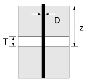
- D: is the pile diameter in meters (see Fig. 2)
- z: is the depth to the bottom of the liquefied layer (see Fig. 2)
- T: is the thickness of the liquefied layer (see Fig. 2)
- phi: is the friction angle of the stronger soil layers in degrees
- gamma: is the unit weight of the stronger soil layers in kN/m^3
- pileE: is the elastic modulus of the deep foundation in kPa
- pileNu: is Poisson's ratio for the deep foundation
- nNode: is the number of desired pile nodes (Note: more than 200 nodes will require modification to the script)
- H: is the length of the pile and soil profile in meters
The scripts create the input file based on the supplied geometry and constitutive parameters. The p-y springs are given constitutive behavior based on the methods discussed above. The resulting input file will be located inside a directory with a matching name.
Results
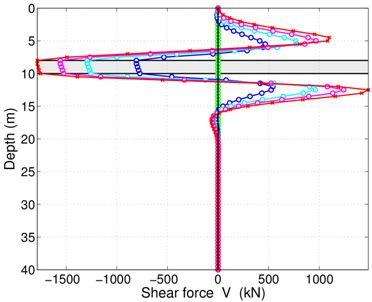
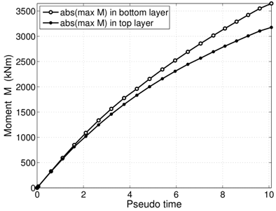
Several plots are provided below to demonstrate the type of results which can be obtained from this analysis and to allow the user to verify the proper implementation of the example input file. Figs. 3 and 4 show the shear force and bending moment diagrams for the deep foundation during the analysis. These plots include the results for a series of time steps, each represented as a different color, to show how the moment and shear change during the lateral spreading event. Fig. 5 shows the load distribution which is applied to the deep foundation during the application of the imposed displacement profile. Fig. 6 shows the displaced shape of the deep foundation at several time steps during the analysis. Figs. 7 and 8 show the evolution of the absolute magnitude and position of the maximum moments in the upper and lower soil layers. Fig. 8 also shows the evolution of the effective length (L_effective), which is the distance between the two maximum moments. The shaded band in these figures shows the location of the liquefied layer.


References
- American Petroleum Institute (API) (1987). Recommended Practice for Planning, Designing and Constructing Fixed Offshore Platforms. API Recommended Practice 2A(RP–2A), Washington, D.C., 17th edition.
- Boulanger, R.W., Kutter, B.L., Brandenberg, S.J., Singh, P., and Chang, D. (2003). Pile foundations in liquefied and laterally spreading ground during earthquakes: Centrifuge experiments and analyses. Center for Geotechnical Modeling, University of California at Davis, Davis, CA. Rep. UCD/CGM-03/01.
- Brandenberg, S.J., Boulanger, R.W., Kutter, B.L., and Chang, D. (2007). "Static pushover analyses of pile groups in liquefied and laterally spreading ground in centrifuge tests." Journal of Geotechnical and Geoenvironmental Engineering, ASCE, 133(9), 1055–1066.
- Brinch Hansen, J. (1961). "The ultimate resistance of rigid piles against transversal forces." Bulletin No. 12, Geoteknisk Institute, Copenhagen, 5–9.
- McGann, C.R., Arduino, P., and Mackenzie-Helnwein, P. (2011). "Applicability of conventional p-y relations to the analysis of piles in laterally spreading soil." Journal of Geotechnical and Geoenvironmental Engineering, ASCE, 137(6), 557-567.
- McGann, C.R., Arduino, P., and Mackenzie-Helnwein, P. (2012). "Simplified procedure to account for a weaker soil layer in lateral load analysis of single piles." Journal of Geotechnical and Geoenvironmental Engineering, ASCE, 138(9), 1129-1137.