Calibration of Maxwell Material
Example posted by: Dimitrios G. Lignos, Ph.D., McGill University
This example demonstrates how to conduct a calibration of a viscous damper using the maxwell model.
The files needed to analyze this structure in OpenSees are included here:
- The main file: Maxwell_Calibrator.tcl
Supporting procedure files
- SquareSsection.tcl – displays a square fiber section
- Damper.txt – contains the displacement loading history of the damper in units of mm
All files are available in a compressed format here: Calibration_Maxwell_example.zip
The rest of this example describes the model and shows the analysis results.
Model Description

The viscous damper is modeled with the nonlinearBeamColumn element. This element follow a Maxwell hysteretic response. An idealized schematic of the model is presented in Figure 1.
The units of the model are mm, kN, and seconds.
Basic Geometry
The basic geometry of the viscous damper is defined by input variables for the length L=5000mm, and area A = 12000mm2. Two nodes are used for the geometry of the damper.
Damper Section
A square section is used to define the area A of the damper (Adamper = 10000.0mm2).
Damper Links
nonlinearBeamColumn elements are used to link the two nodes that define the geometry of the viscous damper with n=5 sections of integration and the damper section defined previously.
Constraints
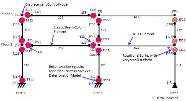
The frame columns are fixed at the base, and the leaning column is pinned at the base. To simulate a rigid diaphragm, the horizontal displacements of all nodes in a given floor are constrained to the leftmost beam-column joint node using the equalDOF command.
Loading
Gravity loads are assigned to the beam-column joint nodes using the nodal load command. Gravity loads tributary to the frame members are assigned to the frame nodes while the remaining gravity loads are applied to the leaning columns. The gravity loads are applied as a plain load pattern with a constant time series since the gravity loads always act on the structure.
In this example, lateral loads are distributed to the frame using the methodology of ASCE 7-10 (http://www.asce.org/Product.aspx?id=2147487569). Lateral loads are applied to all the frame nodes in a given floor. A plain load pattern with a linear time series is used for lateral load application so that loads increase with time.
Recorders
The recorders used in this example include:
- The drift recorder to track the story and roof drift histories
- The node recorder to track the base shear reaction history
- The element recorder to track the element forces in the first story columns as well as the moment and rotation histories of the springs in the concentrated plasticity model
To record the moment and rotation histories in the springs, the region command was used to assign all column springs to one group and all beam springs to a separate group, and the region was used as an input to the element recorder.
It is important to note that the recorders only record information for analyze commands that are called after the recorder commands are called. In this example, the recorders are placed after the gravity analysis so that the steps of the gravity analysis do not appear in the output files.
Analysis
The structure is first analyzed under gravity loads before the pushover analysis is conducted. The gravity loads are applied using a load-controlled static analysis with 10 steps. So that the gravity loads remain on the structure for all subsequent analyses, the loadConst command is used after the gravity analysis is completed. This command is also used to reset the time to zero so that the pushover starts from time zero.
The pushover analysis is performed using a displacement-controlled static analysis. In this example, the structure was pushed to 10% roof drift, or 32.4”. The roof node at Pier 1, node 13 in Figures 1 and 2, was chosen as the control node where the displacement was monitored. Incremental displacement steps of 0.01” were used. This step size was used because it is small enough to capture the progression of hinge formation and generate a smooth backbone curve, but not too small that it makes the analysis time unreasonable.
Results
Comparison of OpenSees Models

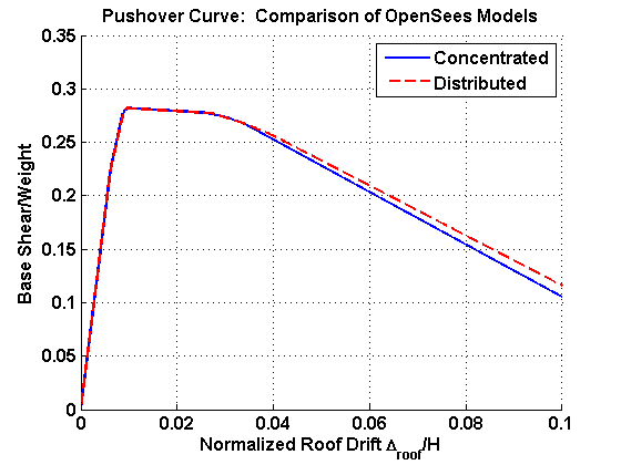
Theoretically, the results of the distributed plasticity model should approach those of the concentrated plasticity model as the length of the plastic hinge regions approaches zero. Because of localized instability due to the stress-strain formulation of the beam with hinges element, the distributed plasticity model does not give reasonable results when the length of the plastic hinge is very small (i.e., 10e-5). Therefore, the length of the plastic hinges was increased from 10e-5 until the results of this model approached those of the concentrated plasticity model. The plastic hinge length that led to agreement between the models was 0.4% of the frame member's total length. The periods of the concentrated and distributed models are very close: T1 = 0.83 s (con) vs. 0.82 s (dist) and T2 = 0.22 s (con) vs. 0.21 s (dist).
The results of the pushover analyses from the OpenSees models are shown in Figure 3. This figure shows the normalized base shear (weight of the structure divided by the base shear) versus the roof drift (roof displacement divided by the roof elevation). The models are nearly identical until about 2.5% roof drift when their curves begin to diverge. The descending branch of the the concentrated plasticity model is slightly steeper, but the two models agree reasonably well as there is less than 10% percent difference in the base shears at 10% roof drift.
References
- Ibarra, L. F., and Krawinkler, H. (2005). “Global collapse of frame structures under seismic excitations,” Technical Report 152, The John A. Blume Earthquake Engineering Research Center, Department of Civil Engineering, Stanford University, Stanford, CA. [electronic version: https://blume.stanford.edu/tech_reports]
- Ibarra, L. F., Medina, R. A., and Krawinkler, H. (2005). “Hysteretic models that incorporate strength and stiffness deterioration,” Earthquake Engineering and Structural Dynamics, Vol. 34, 12, pp. 1489-1511.
- Lignos, D. G., and Krawinkler, H. (2009). “Sidesway Collapse of Deteriorating Structural Systems under Seismic Excitations,” Technical Report 172, The John A. Blume Earthquake Engineering Research Center, Department of Civil Engineering, Stanford University, Stanford, CA.
- Lignos, D. G., and Krawinkler, H. (2010). “Deterioration Modeling of Steel Beams and Columns in Support to Collapse Prediction of Steel Moment Frames,” ASCE, Journal of Structural Engineering (under review).