Simply supported beam modeled with two dimensional solid elements
Example Provided by: Vesna Terzic, UC Berkeley
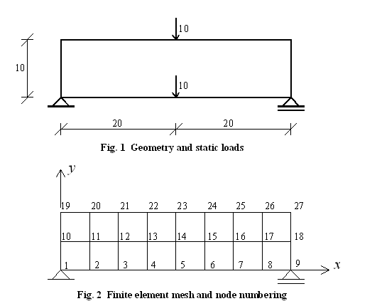
This example (adopted from the old OpenSees Examples Manual) considers a simple problem in solid dynamics. The structure is a simply supported beam modelled with two dimensional solid elements (quadrilateral elements). The beam is first exposed to static load (two nodal loads) and then to free vibrations caused by removal of the static load. Free vibrations of the beam are graphically displayed at the time the beam is analyzed. Three types of quadrilateral elements: quad element, bbarQuad element, and enhencedQuad element are considered in analysis and their results are compared.
Fig. 1 shows the geometry of the beam and the static load. Units adopted for this example are: kip, inch, sec. Fig. 2 shows the global coordinate system, finite element mesh, and nodal numeration.
Instructions on how to run this example
To execute this ananlysis in OpenSees download this file: DynAnal_BeamWithQuadElements.tcl
To run this example, place the OpenSees.exe to the same directory with the downloaded file. By double cliking on OpenSees.exe the OpenSees interpreter will pop out. To run the analysis the user sholud type "source Example6_1.tcl" in OpenSees interpreter and hit enter.
Create the model
Spatial dimension of the model and number of degrees-of-freedom (DOF) at nodes are defined using model command. For two-dimensional analysis, a typical solid element is defined as a volume in two-dimensional space. In this example we have 2D model with 2 DOFs at each node. This is defined in the following way:
model BasicBuilder -ndm 2 -ndf 2
The geometry of the beam will be defined and the mesh of quadrilateral elements will be generated using bloc2D command. This command also specifies the type of quadrilateral elements to be used in analysis. In order to define a quadrilateral element we need to create the NDmaterial first. For this example ElasticIsotropic material is used.
nDMaterial ElasticIsotropic 1 1000 0.25 6.75
Choose the type of quadrilateral element to use in the analysis:
set Quad quad
or
set Quad bbarQuad
or
set Quad enhancedQuad
Arguments for the three types of quadrilateral elements under consideration are defined next. All three elements model plane strain material behavior.
if {$Quad == "enhancedQuad" } {
	set eleArgs "PlaneStrain2D 1"
}
if {$Quad == "quad" } {
	set eleArgs "1 PlaneStrain2D 1"
}
if {$Quad == "bbarQuad" } {
	set eleArgs "1"
}
Number of elements in x and y direction of the beam are set to:
set nx 8
set ny 2
The user can change these values and make the mesh finer or coarser. Number of elements in x direction has to remain even since the forces are applied at the beam centerline.
The nodes and elements are defined next using block2D command.
block2D $nx $ny 1 1 $Quad $eleArgs {
	1  0   0
	2  40  0
	3  40  10
	4  0   10
}
The boundary conditions are defined next using single-point constraint command fix. Node 1 is fixed in both direction and node bn is a roller.
fix 1 1 1 1;
fix 2 1 1 1;
Masses are assigned at nodes 3, 4, 5, and 6 using mass command. Since the considered shear frame system has only two degrees of freedom (displacements in x at the 1st and the 2nd storey), the masses have to be assigned in x direction only.
mass 3 $m 0. 0. ;
mass 4 $m 0. 0. ;
mass 5 [expr $m/2.] 0. 0. ;
mass 6 [expr $m/2.] 0. 0. ;
The geometric transformation with id tag 1 is defined to be linear.
set TransfTag 1;
geomTransf Linear $TransfTag ;
The beams and columns of the frame are defined to be elastic using elasticBeamColumn element. In order to make beams infinitely rigid moment of inertia for beams (Ib) is set to very high value (10e+12).
element elasticBeamColumn 1 1 3 $Ac $Ec [expr 2.*$Ic] $TransfTag;
element elasticBeamColumn 2 3 5 $Ac $Ec $Ic           $TransfTag;
element elasticBeamColumn 3 2 4 $Ac $Ec [expr 2.*$Ic] $TransfTag;
element elasticBeamColumn 4 4 6 $Ac $Ec $Ic           $TransfTag;
element elasticBeamColumn 5 3 4 $Ab $E  $Ib           $TransfTag;
element elasticBeamColumn 6 5 6 $Ab $E  $Ib           $TransfTag;
To comply with the assumptions of the shear frame (no vertical displacemnts and rotations at nodes) end nodes of the beams are constrained to each other in the 2nd DOF (vertical displacement) and the 3rd DOF (rotation). EqualDOF command is used to imply these constraints.
equalDOF 3 4 2 3
equalDOF 5 6 2 3
Define recorders
For the specified number of eigenvalues (numModes) (for this example it is 2) the eigenvectors are recorded at all nodes in all DOFs using node recorder command.
for { set k 1 } { $k <= $numModes } { incr k } {
    recorder Node -file [format "modes/mode%i.out" $k] -nodeRange 1 6 -dof 1 2 3  "eigen $k"
}
Perform eigenvalue analysis
The eigenvalues are calculated using eigen commnad and stored in lambda variable.
set lambda [eigen $numModes];
Display mode shapes
As there are two mode shapes of the system we will create two display windows using record display command. Here we specify window title (e.g., "Mode Shape 1"), then x and y location of the top-left corner of the window (relative to the upper-left corner of the screen), and finally width and height of the graphical window in pixels. Projector reference point (prp) is defined next. This point defines the center of projection (viewer's eye). Usually it is placed at the center of the object that is to be graphically presented. For this example, the center of the structure is at (h,h), h being the height of the column (Figure 1). Next, we have to define view-up (vup) vector and view-plane normal (vpn) vector. They are (0,1,0) and (0,0,1), respectively. Window view is defined next using command viewWindow and the four coordinates (-x, x, -y, y) that define the size of the viewing window relative to the prp. In this example h is 144, so the viewing window with its vector (-200, 200, -200, 200) is set to have 56 units of blank space all around the structure. Finally, we use display command to display the mode shapes. The first argument following the command specifies the type of response to be plotted (e.g., -1 is tag for displaying the 1st mode shape, -2 is the tag for displaying the 2nd mode shape, and so on). The second argument following display command is magnification factor for nodes and the third argument is magnification factor for the response quantity to be displayed.
recorder display "Mode Shape 1" 10 10 500 500 -wipe
prp $h $h 1;
vup  0  1 0;
vpn  0  0 1;
viewWindow -200 200 -200 200
display -1 5 20

recorder display "Mode Shape 2" 10 510 500 500 -wipe
prp $h $h 1;
vup  0  1 0;
vpn  0  0 1;
viewWindow -200 200 -200 200
display -2 5 20
One step of analysis with no loading
In order to record any response quantity in OpenSess (in this example we want to record eigenvectors) at least one step of analysis has to be performed. Analysis objects are defined and one step of analysis is performed.
integrator LoadControl 0 1 0 0
test EnergyIncr	       1.0e-10    100        0
algorithm Newton
numberer RCM
constraints Transformation
system ProfileSPD
analysis Static

analyze 1