Laterally-Loaded Pile Foundation
Example Provided by: Christopher McGann, University of Washington
This article describes the OpenSees implementation of a simple laterally-loaded pile example. The problem is modeled as a beam on a nonlinear Winkler foundation (BNWF), utilizing displacement-based beam elements for the pile and nonlinear spring elements which represent the vertical and lateral response of the surrounding soil.
Provided with this article are the files needed to execute this analysis in OpenSees;
- the main input file, staticBNWFpile.tcl
- three procedures to define the soil constitutive behavior, get_pyParam.tcl, get_tzParam.tcl, and get_qzParam.tcl
- a file to define the pile section behavior, elasticSection.tcl
To run this example, the user must download each of the above files and place them in a single directory. Once this has been done, the user can then type "source staticBNWFpile.tcl" into the interpreter of the OpenSees.exe application to run the analysis. Representative results are presented in this article to verify the correct implementation of this example. Additionally, the pile response obtained from this analysis is compared to a similar analysis conducted using the commercial program LPile (http://www.ensoftinc.com) to provide verification the results of the OpenSees analysis.
Model Description

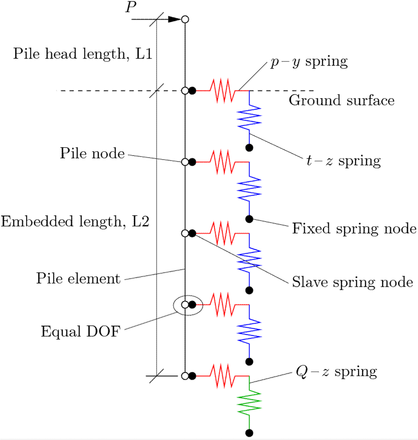
The BNWF model simulates the laterally-loaded pile problem using displacement-based beam elements to represent the pile and a series of nonlinear springs to represent the soil. The soil springs are generated using zero-length elements assigned separate uniaxial material objects in the lateral and vertical directions. An idealized schematic of the laterally-loaded pile model is provided in Fig. 1.
The pile axis is oriented in the z-coordinate direction, and all of the nodes are initially located on the z-axis (x- and y- coordinates are zero). The model is created with three separate sets of nodes:
- fixed spring nodes (numbers 1-85 in example)
- slave spring nodes (numbers 101-185 in example)
- pile nodes (numbers 201-285 in example)
Geometry and Mesh
The geometry is rather simple in this example. There is only a single layer of cohesionless soil, and the groundwater table is assumed to be well below the tip of the pile. The pile geometry controls the meshing of the problem. The user can specify the length of the pile head (above the ground surface), L1, and the embedded pile length (below the ground surface), L2. The default values in staticBNWFpile.tcl are L1 = 1 m, and L2 = 20 m.
The mesh is defined by the number of elements specified in the pile. The default value in this example is 84 elements (85 nodes). For the default pile geometry, this results in 80 elements over the embedded length and 4 elements above the ground surface. The input file is set up to handle up to 100 nodes. Modifications would need to be made to the node numbering scheme to accommodate a larger number of nodes.
Spring Nodes
The spring nodes are created with three dimensions and three translational degrees-of-freedom (dof). The input file is set up to automatically generate the necessary spring nodes and elements based upon the input geometry (pile head length, $L1, embedded length, $L2, and number of pile elements, $nElePile). Spring nodes are only created over the embedded length of pile.
Since zero-length elements are used for the springs, the two sets of nodes share the same set of locations. One set of spring nodes, the fixed-nodes, are initially fixed in all three dof. The other set of nodes, the slave nodes, are initially fixed in only two dof, and are later given equal dof with the pile nodes.
Spring Constitutive Behavior
The constitutive behavior of the springs is defined such that the springs oriented in the lateral direction represent p-y springs, and the vertically-oriented springs represent t-z and Q-z springs for the pile shaft and tip, respectively. Three procedures are used to properly define the p-y/t-z/Q-z behavior with depth.
Several input soil properties are necessary to define these springs:
- soil unit weight, $gamma
- soil internal friction angle, $phi
- soil shear modulus, $Gsoil
The default values are set at $gamma = 17 kN/m^3, $phi = 36 degrees, and $Gsoil = 150000 kPa.
The procedure get_pyParam.tcl, which defines the p-y springs, has several options which must be selected.
- The first switch, $puSwitch, specifies the variation in ultimate lateral resistance with depth. The default, $puSwitch = 1, uses the recommendations of the American Petroleum Institute (API) (1993). The alternative method is that of Brinch Hansen (1961).
- The second switch, $kSwitch, specifies the variation in initial stiffness with depth. The default, $kSwitch = 1, specifies a linear variation of initial stiffness with depth (API 1993). The alternative uses a modified version of the API stiffness which varies parabolically with depth after Boulanger et al. (2003).
- The presence of groundwater can be accounted for in the initial stiffness using the third switch, $gwtSwitch. Default, $gwtSwitch = 1, is for no groundwater.
The p-y spring constitutive behavior is obtained using the PySimple1 uniaxial material object. The t-z and Q-z springs are defined using the TzSimple1 and QzSimple1 uniaxial materials, respectively. The main input file is set up to automatically generate the required spring material objects based upon the input geometry and soil properties.
Spring Elements
Zero-length elements are used for the soil springs using the element zeroLength. These elements connect the fixed and slave spring nodes. The the PySimple1 material objects are incorporated in dof 1 (direction of loading), while the TzSimple1, and at the pile tip, the QzSimple1, material objects are incorporated in dof 3 (vertical direction).