LeadRubberX
This command is used to construct a LeadRubberX bearing element object in three-dimension. The 3D continuum geometry of a lead rubber bearing is modeled as a 2-node, 12 DOF discrete element. It extends the formulation of ElastomericX by including strength degradation in lead rubber bearing due to heating of lead-core. The LeadRubberX element requires only the geometric and material properties of an elastomeric bearing as arguments. The material models in six direction are formulated within the element from input arguments.
For a 3D problem:
| element LeadRubberX $eleTag $Nd1 $Nd2 $qLead $uh $Gr $Kbulk $D1 $D2 $ts $tr $n <<$x1 $x2 $x3> $y1 $y2 $y3> <$kc> <$PhiM> <$ac> <$sDratio> <$m> <$cd> <$tc> <$qL> <$cL> <$kS> <$aS> <$tag1> <$tag2> <$tag3> <$tag4> <$tag5> |
| $eleTag | unique element object tag |
| $Nd1 $Nd2 | end nodes |
| $qLead | yield strength |
| $uh | yield deformation |
| $Gr | shear modulus of elastomeric bearing |
| $Kbulk | bulk modulus of rubber |
| $D1 | internal diameter |
| $D2 | outer diameter (excluding cover thickness) |
| $ts | single steel shim layer thickness |
| $tr | single rubber layer thickness |
| $n | number of rubber layers |
| $x1 $x2 $x3 | vector components in global coordinates defining local x-axis (optional) |
| $y1 $y2 $y3 | vector components in global coordinates defining local y-axis (optional) |
| $kc | cavitation parameter (optional, default = 10.0) |
| $PhiM | damage parameter (optional, default = 0.5) |
| $ac | strength reduction parameter (optional, default = 1.0) |
| $sDratio | shear distance from iNode as a fraction of the element length (optional, default = 0.5) |
| $m | element mass (optional, default = 0.0) |
| $cd | viscous damping parameter (optional, default = 0.0) |
| $tc | cover thickness (optional, default = 0.0) |
| $qL | density of lead (optional, default = 11200 kg/m3) |
| $cL | specific head of lead (optional, default = 130 N-m/kg oC) |
| $kS | thermal conductivity of steel (optional, default = 50 W/m oC) |
| $aS | thermal diffusivity of steel (optional, default = 1.41e-05 m2/s) |
| $tag1 | Tag to include cavitation and post-cavitation (optional, default = 0) |
| $tag2 | Tag to include buckling load variation (optional, default = 0) |
| $tag3 | Tag to include horizontal stiffness variation (optional, default = 0) |
| $tag4 | Tag to include vertical stiffness variation (optional, default = 0) |
| $tag5 | Tag to include strength degradation in shear due to heating of lead core (optional, default = 0) |
Important note:
Because default values of heating parameters are in SI units, user must override the default heating parameters values if using Imperial units
Physical Model and Mechanical Properties
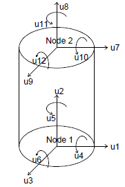
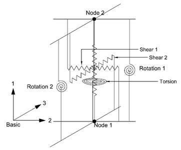
The physical model of an elastomeric bearing is considered as a two-node, twelve degrees-of-freedom discrete element. The two nodes are connected by six springs that represent the mechanical behavior in the six basic directions of a bearing. The degrees of freedom and discrete spring representation of an elastomeric bearing are shown in the below figures.
The general form of element force vector, <math>{{f}_{b}}</math>, and element stiffness matrix,<math>{{K}_{b}}</math> , for element representation considered above is given by equation below:
<math>{{f}_{b}}=\left[ \begin{matrix}
  Axial  \\
  Shear1  \\
  Shear2  \\
  Torsion  \\
  Rotation1  \\
  Rotation2  \\
\end{matrix} \right];\ \ \ \ \ \ {{K}_{b}}=\left[ \begin{matrix}
  Axial & 0 & 0 & 0 & 0 & 0  \\
  0 & Shear1 & Shear12 & 0 & 0 & 0  \\
  0 & Shear21 & Shear2 & 0 & 0 & 0  \\
  0 & 0 & 0 & Torsion & 0 & 0  \\
  0 & 0 & 0 & 0 & Rotation1 & 0  \\
  0 & 0 & 0 & 0 & 0 & Rotation2  \\
\end{matrix} \right]</math>
The coupling of the two shear springs is considered directly by using a coupled bidirectional model. All other springs are uncoupled. The coupling of vertical and horizontal directions are considered indirectly by using expressions for mechanical properties in one direction that are dependent on the response parameters in the other direction. Linear uncoupled springs are considered in the torsion and the two rotational springs as they are not expected to significantly affect the response of an elastomeric bearing. The off-diagonal terms due to coupling between axial and shear, and axial and rotation, are not considered in the two-spring model (Koh and Kelly, 1987) used here. An exact model would have non-zero values of these off-diagonal terms. A discussion on the formulation of the two-spring model and the exact model is presented in Ryan et al.(1991). The subscript b refers to the element’s basic coordinate system. When the model is implemented in software programs, response quantities are transformed between the basic, local and global coordinates to perform computations.
The discrete spring model presented here has the advantages of easy implementation and being computationally efficient. The mechanical properties of the six springs (also referred to as material models in OpenSees) are defined using analytical solutions available from the analysis of elastomeric bearings. The expression for mechanical properties, including stiffness and buckling load capacity, are derived using explicit consideration for geometric nonlinearity due to large displacement effects. The P-Delta effect, which is an approximate method to account for geometric nonlinearity in structural analysis problems, is therefore not considered. The material models in six directions are:
- Axial direction: a new mathematical model that captures the behavior under cyclic tension Link
- Two shear directions: a special case of the Bouc-Wen model extended by Nagarajaiah et al.(1991) for seismic isolation bearings combined with a strength degradation model of Kalpakidis et al.(2010)
- Torsion: a linear elastic model
- Two rotational directions: linear elastic models
In addition to the behavior captured by existing bearing elements, this element can capture following characteristics:
- Cavitation and post-cavitation behavior in tension (tag1)
- Variation in critical buckling load capacity due to lateral displacement (tag2)
- Variation in horizontal shear stiffness with axial load on the bearing (tag3)
- Variation in vertical axial stiffness with horizontal displacement (tag4)
- Strength degradation in cyclic shear loading due to heating of lead core (tag5)
User may choose to include an individual or a combination of these behaviors through user tags (include:1, exclude:0) in their analysis.
For the full capabilities of this element, users are referred to: EESD Article
Examples
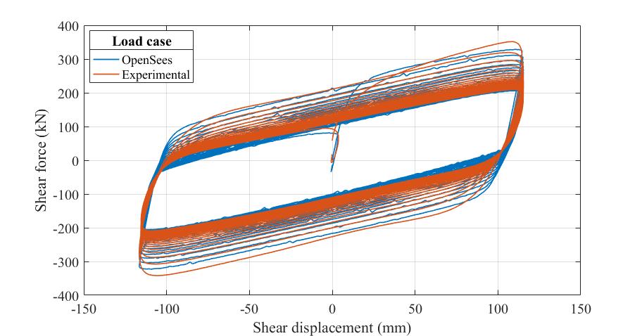
An example is presented here in which a lead rubber bearing (large size bearing in Kalpakidis et al. (2010)) is subjected to a shear harmonic loading in laboratory (SEESL at UB). The response obtained from LeadRubberX element in OpenSees is compared with the experimental results.
Excitation files: File:Excitation.zip
Tcl files: File:LDRgravity.tcl File:LDRtest.tcl
References
- Kumar, M., Whittaker, A., and Constantinou, M. (2014). "An advanced numerical model of elastomeric seismic isolation bearings." Earthquake Engineering & Structural Dynamics, Published online, DOI: 10.1002/eqe.2431. Link
- Kalpakidis, I. V., Constantinou, M. C., and Whittaker, A. S. (2010). "Modeling strength degradation in lead-rubber bearings under earthquake shaking." Earthquake Engineering and Structural Dynamics, 39(13), 1533-1549.
Code Developed by: Manish Kumar, University at Buffalo, SUNY.
Any bugs in this element can be reported to mkumar2 AT buffalo dot edu


