Time History Analysis of a 2D Elastic Cantilever Column: Difference between revisions
(Created page with 'This page is under construction... Example Provided by: <span style="color:blue"> Vesna Terzic, UC Berkeley</span> ---- This example demonstrates how to perform time hystory a...') |
No edit summary |
||
| Line 5: | Line 5: | ||
---- | ---- | ||
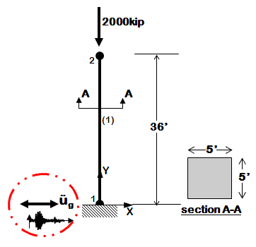
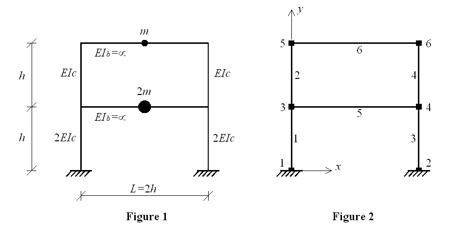
This example demonstrates how to perform time | This example demonstrates how to perform time history analysis of a 2D elastic cantilever column. This is a tutorial for the Ex1a.Canti2D.EQ.tcl (given in the [[Examples Manual|examples manual]]) and is intended to help beginners with OpenSees. Idealized two-storey shear frame (Example 10.4 from "Dynamic of Structures" book by Professor Anil K. Chopra) is used for this purpose. In this idealization beams are rigid in flexure, axial deformation of beams and columns are neglected, and the effect of axial force on the stiffness of the columns is neglected. Geometry and material characteristics of the frame structure are shown in Figure 1. Node and element numbering is given in Figure 2. | ||
---- | ---- | ||
|- | |- | ||
[[File:Example1a_EQ.GIF|link=OpenSees Example 1a. 2D Elastic Cantilever Column]] | [[File:Example1a_EQ.GIF|link=OpenSees Example 1a. 2D Elastic Cantilever Column]] | ||
---- | ---- | ||
Revision as of 20:57, 24 September 2010
This page is under construction...
Example Provided by: Vesna Terzic, UC Berkeley
This example demonstrates how to perform time history analysis of a 2D elastic cantilever column. This is a tutorial for the Ex1a.Canti2D.EQ.tcl (given in the examples manual) and is intended to help beginners with OpenSees. Idealized two-storey shear frame (Example 10.4 from "Dynamic of Structures" book by Professor Anil K. Chopra) is used for this purpose. In this idealization beams are rigid in flexure, axial deformation of beams and columns are neglected, and the effect of axial force on the stiffness of the columns is neglected. Geometry and material characteristics of the frame structure are shown in Figure 1. Node and element numbering is given in Figure 2.
|-
Instructions on how to run this example
To execute this ananlysis in OpenSees download this file: EigenAnal_twoStoreyShearFrame.tcl
To run this example, place the OpenSees.exe to the same directory with the downloaded file. By double cliking on OpenSees.exe the OpenSees interpreter will pop out. To run the analysis the user sholud type "source EigenAnal_twoStoreyShearFrame7.tcl" in OpenSees interpreter and hit enter. To create output files of eigenvectors (stored in directory "modes") the user has to exit OpenSees interpreter by typing "exit".
Create the model
Spatial dimension of the model and number of degrees-of-freedom (DOF) at nodes are defined using model command. In this example we have 2D model with 3 DOFs at each node. This is defined in the following way:
model BasicBuilder -ndm 2 -ndf 3
Note: geometry, mass, and material characteristics are assigned to variables that correspond to the ones shown in Figure 1 (e.g., the height of the column is set to be 144 in. and assigned to variable h; the value of the height can be accessed by $h).
Nodes of the structure (Figure 2) are defined using the node command:
node 1   0.  0. ;
node 2   $L  0. ;
node 3   0.  $h ;
node 4   $L  $h ;
node 5   0.  [expr 2*$h];
node 6   $L  [expr 2*$h];
The boundary conditions are defined next using single-point constraint command fix. In this example nodes 1 and 2 are fully fixed at all three DOFs:
fix 1 1 1 1;
fix 2 1 1 1;
Masses are assigned at nodes 3, 4, 5, and 6 using mass command. Since the considered shear frame system has only two degrees of freedom (displacements in x at the 1st and the 2nd storey), the masses have to be assigned in x direction only.
mass 3 $m 0. 0. ;
mass 4 $m 0. 0. ;
mass 5 [expr $m/2.] 0. 0. ;
mass 6 [expr $m/2.] 0. 0. ;
The geometric transformation with id tag 1 is defined to be linear.
set TransfTag 1;
geomTransf Linear $TransfTag ;
The beams and columns of the frame are defined to be elastic using elasticBeamColumn element. In order to make beams infinitely rigid moment of inertia for beams (Ib) is set to very high value (10e+12).
element elasticBeamColumn 1 1 3 $Ac $Ec [expr 2.*$Ic] $TransfTag;
element elasticBeamColumn 2 3 5 $Ac $Ec $Ic           $TransfTag;
element elasticBeamColumn 3 2 4 $Ac $Ec [expr 2.*$Ic] $TransfTag;
element elasticBeamColumn 4 4 6 $Ac $Ec $Ic           $TransfTag;
element elasticBeamColumn 5 3 4 $Ab $E  $Ib           $TransfTag;
element elasticBeamColumn 6 5 6 $Ab $E  $Ib           $TransfTag;
To comply with the assumptions of the shear frame (no vertical displacemnts and rotations at nodes) end nodes of the beams are constrained to each other in the 2nd DOF (vertical displacement) and the 3rd DOF (rotation). EqualDOF command is used to imply these constraints.
equalDOF 3 4 2 3
equalDOF 5 6 2 3
Define recorders
For the specified number of eigenvalues (numModes) (for this example it is 2) the eigenvectors are recorded at all nodes in all DOFs using node recorder command.
for { set k 1 } { $k <= $numModes } { incr k } {
    recorder Node -file [format "modes/mode%i.out" $k] -nodeRange 1 6 -dof 1 2 3  "eigen $k"
}
Perform eigenvalue analysis
The eigenvalues are calculated using eigen commnad and stored in lambda variable.
set lambda [eigen $numModes];
The periods and frequencies of the structure are calculated next.
set omega {}
set f {}
set T {}
set pi 3.141593

foreach lam $lambda {
	lappend omega [expr sqrt($lam)]
	lappend f [expr sqrt($lam)/(2*$pi)]
	lappend T [expr (2*$pi)/sqrt($lam)]
}
The periods are stored in a Periods.txt file inside of directory "modes".
set period "modes/Periods.txt"
set Periods [open $period "w"]
foreach t $T {
	puts $Periods " $t"
}
close $Periods
Display mode shapes
As there are two mode shapes of the system we will create two display windows using record display command. Here we specify window title (e.g., "Mode Shape 1"), then x and y location of the top-left corner of the window (relative to the upper-left corner of the screen), and finally width and height of the graphical window in pixels. Projector reference point (prp) is defined next. This point defines the center of projection (viewer's eye)(for more information: Viewpoint Projections and Specifications). Usually it is placed at the center of the object that is to be graphically presented. For this example, the center of the structure is at (h,h), h being the height of the column (Figure 1). Next, we have to define view-up (vup) vector and view-plane normal (vpn) vector. They are (0,1,0) and (0,0,1), respectively. Window view is defined next using command viewWindow and the four coordinates (-x, x, -y, y) that define the size of the viewing window relative to the prp. In this example h is 144, so the viewing window with its vector (-200, 200, -200, 200) is set to have 56 units of blank space all around the structure. Finally, we use display command to display the mode shapes. The first argument following the command specifies the type of response to be plotted (e.g., -1 is tag for displaying the 1st mode shape, -2 is the tag for displaying the 2nd mode shape, and so on). The second argument following display command is magnification factor for nodes and the third argument is magnification factor for the response quantity to be displayed.
recorder display "Mode Shape 1" 10 10 500 500 -wipe
prp $h $h 1;
vup  0  1 0;
vpn  0  0 1;
viewWindow -200 200 -200 200
display -1 5 20

recorder display "Mode Shape 2" 10 510 500 500 -wipe
prp $h $h 1;
vup  0  1 0;
vpn  0  0 1;
viewWindow -200 200 -200 200
display -2 5 20
One step of analysis with no loading
In order to record any response quantity in OpenSess (in this example we want to record eigenvectors) at least one step of analysis has to be performed. Analysis objects are defined and one step of analysis is performed.
integrator LoadControl 0 1 0 0
test EnergyIncr	       1.0e-10    100        0
algorithm Newton
numberer RCM
constraints Transformation
system ProfileSPD
analysis Static

analyze 1