Moment Curvature Example: Difference between revisions
(Created page with '__NOTOC__ This next example covers the moment-curvature analysis of a rectangular reinforced concrete section. In this example a Zero Length element with the fiber discretization...') |
No edit summary |
||
| (10 intermediate revisions by the same user not shown) | |||
| Line 2: | Line 2: | ||
This next example covers the moment-curvature analysis of a rectangular reinforced concrete section. In this example a Zero Length element with the fiber discretization of the cross section is used. In addition to providing understanding as to the creation of a fiber section, the example introduces Tcl language features such as variable and command substitution, expression evaluation and the use of procedures. | This next example covers the moment-curvature analysis of a rectangular reinforced concrete section. In this example a Zero Length element with the fiber discretization of the cross section is used. In addition to providing understanding as to the creation of a fiber section, the example introduces Tcl language features such as variable and command substitution, expression evaluation and the use of procedures. | ||
Here is the file: [[Media:MomentCurvature.tcl | MomentCurvature.tcl]] | |||
[[Image:MomentCurvature.png|link=Moment Curvature Example]] | [[Image:MomentCurvature.png|link=Moment Curvature Example]] | ||
| Line 12: | Line 12: | ||
=== Tcl Basics === | === Tcl Basics === | ||
In the script that is to be presented variables are to be used. | In the tcl script that is to be presented, variables, expressions and procedures are used. | ||
the syntax of $variable. Expressions can be evaluated, | |||
A variable is a symbolic name given to some known or unknown quantity or information, for the purpose of allowing the name to be used independently of the information it represents. In Tcl a variable once set (with the set command) can then be subsequently using the syntax of $variable. The following tcl example sets the variable v to be 2.0, and then prints to the screen a message saying what the value of v is. | |||
result of an expression is then set to another variable. A simple example to add 2.0 to a | |||
<pre> | |||
set v 3.0 | |||
puts "v equals $v" | |||
</pre> | |||
Expressions can be evaluated using the expr command. When using the expr command, most mathematical functions found in any programming language can be used, e.g. sin(), cos(), max(), min(), abs(),... It is also typical to combine an expression command, with a set command. To do this, the expr command is enclosed in square brackets []'s. The following example demonstrates the setting of a variable v to be 3.0, the setting of another variable sum to be the result of adding whatever the value of the variable v is to 2.0, and finally the printing to the screen of a message saying what the current value of sum is. | |||
Typically, the result of an expression is then set to another variable. A simple example to add 2.0 to a | |||
parameter and print the result is shown below: | parameter and print the result is shown below: | ||
| Line 21: | Line 30: | ||
set v 3.0 | set v 3.0 | ||
set sum [expr $v + 2.0] | set sum [expr $v + 2.0] | ||
puts $sum; # print the sum | puts "sum equals $sum"; # print the sum | ||
</pre> | </pre> | ||
=== Section === | === MomentCurvature.tcl Script === | ||
The file contains 2 parts. The first part contains a procedure named MomentCurvature, and the second part contains the creation of | |||
the section and the subsequent calling of the procedure. | |||
NOTES: | |||
# Typically useful procedures such as MomentCurvature would be placed in a separate file. This is done so that other scripts can also use them. It is only placed in the same file here to limit the number of downloads for the reader of this article. | |||
# In the referenced file, the procedure proceeds the calling of the procedure. It must always be thus. In this article we discuss the section generation first. | |||
=== Section Definition === | |||
For the zero length element, a section discretized by concrete and steel is created to represent the behaviour. UniaxialMaterial objects are created which define the fiber stress-strain relationship's. There is confined concrete in the core, unconfined concrete in the cover region, and reinforcing steel. | For the zero length element, a section discretized by concrete and steel is created to represent the behaviour. UniaxialMaterial objects are created which define the fiber stress-strain relationship's. There is confined concrete in the core, unconfined concrete in the cover region, and reinforcing steel. | ||
[[Image:MomentCurvatureSection.png|link=Moment Curvature Section]] | |||
The dimension of the section are as shown in the figure. The section depth is 24 inches, the width 15 inches, and there is 1.5inch cover all around. Strong axis bending is about the z-axis. The section is separated into confined and unconfined concrete regions, for which separate discretizations will be generated, Reinforcing steel is placed around the boundary of th confined and unconfined regions. The fiber discretization is shown below: | The dimension of the section are as shown in the figure. The section depth is 24 inches, the width 15 inches, and there is 1.5inch cover all around. Strong axis bending is about the z-axis. The section is separated into confined and unconfined concrete regions, for which separate discretizations will be generated, Reinforcing steel is placed around the boundary of th confined and unconfined regions. The fiber discretization is shown below: | ||
[[Image:MomentCurvatureSectionDiscritization.png|link=Moment Curvature Section Discritization]] | |||
The following are the commands that generate the section and perform the moment curvature analysis. The model and analysis commands are contained in the MomentCurvature procedure. These are contained in a seperate file which are "sourced"" by the main script. | The following are the commands that generate the section and perform the moment curvature analysis. The model and analysis commands are contained in the MomentCurvature procedure. These are contained in a seperate file which are "sourced"" by the main script. | ||
| Line 106: | Line 127: | ||
# Call the section analysis procedure | # Call the section analysis procedure | ||
MomentCurvature 1 $P [expr $Ky*$mu] $numIncr | MomentCurvature 1 $P [expr $Ky*$mu] $numIncr | ||
</pre> | </pre> | ||
| Line 113: | Line 133: | ||
=== Moment Curvature Procedure === | === Moment Curvature Procedure === | ||
The Tcl procedure to perform the moment-curvature analysis follows. The | The Tcl procedure to perform the moment-curvature analysis follows. The procedure takes as input the tag of the section to be analyzed, the axial load, P, to be applied, the max curvature to be evaluated and the number of iterations to achieve this max curavature. | ||
The procedure first creates the model which consists of two nodes, boundary conditions, and a ZeroLengthSection element. A depiction of the geometry is as shown in the top most figure above. The image on the left shows an edge view of the element, with local z-axis coming out of the page. Node 1 is completely restrained, with the applied loads acting at Node 2. An axial load, P, is applied to the section during the moment curvature analysis. | |||
After the model has been created, the analysis is performed. A single load step is first performed for the axial load, then the integrator | After the model has been created, the analysis is performed. A single load step is first performed for the axial load, then the integrator | ||
| Line 168: | Line 189: | ||
# Use displacement control at node 2 for section analysis | # Use displacement control at node 2 for section analysis | ||
integrator DisplacementControl 2 3 | integrator DisplacementControl 2 3 $dK | ||
# Do the section analysis | # Do the section analysis | ||
analyze $numIncr | analyze $numIncr | ||
} | } | ||
</pre> | </pre> | ||
| Line 183: | Line 203: | ||
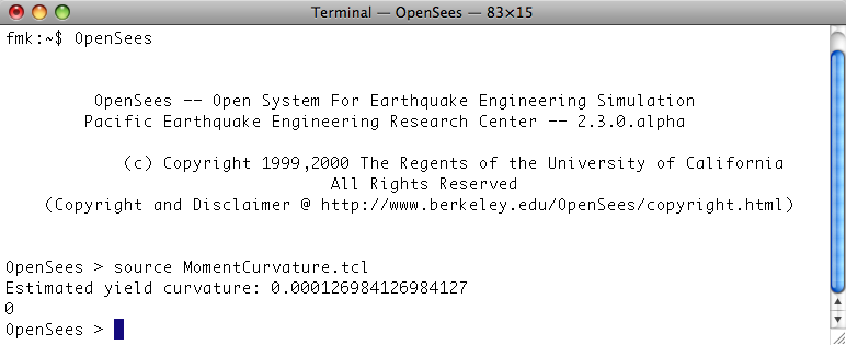
When you run this script, you should see the following printed to the screen: | When you run this script, you should see the following printed to the screen: | ||
[[Image: | [[Image:MomentCurvatureRun.png|link=Moment Curvature Run]] | ||
In addition, your directory should contain the following a file section1.out. A plot of this file using the following matlab commands | |||
<pre> | |||
load section1.out | |||
plot(section1(:,2),sections1(:,1) | |||
xlabel("Curvature 1/in") | |||
ylabel("Moment kip-in") | |||
</pre> | |||
will produce the following: | |||
[[Image:MomentCurvaturePlot.png|link=Moment Curvature Plot]] | |||
Latest revision as of 00:02, 15 April 2011
This next example covers the moment-curvature analysis of a rectangular reinforced concrete section. In this example a Zero Length element with the fiber discretization of the cross section is used. In addition to providing understanding as to the creation of a fiber section, the example introduces Tcl language features such as variable and command substitution, expression evaluation and the use of procedures.
Here is the file: MomentCurvature.tcl
NOTE:
- The lines in the dashed boxes are lines that appear in the input file.
- all lines that begin with # are comments, they are ignored by the program (interpreter) but are useful for documenting the code. When creating your own input scripts you are highly encouraged to use comments.
Tcl Basics
In the tcl script that is to be presented, variables, expressions and procedures are used.
A variable is a symbolic name given to some known or unknown quantity or information, for the purpose of allowing the name to be used independently of the information it represents. In Tcl a variable once set (with the set command) can then be subsequently using the syntax of $variable. The following tcl example sets the variable v to be 2.0, and then prints to the screen a message saying what the value of v is.
set v 3.0
puts "v equals $v"
Expressions can be evaluated using the expr command. When using the expr command, most mathematical functions found in any programming language can be used, e.g. sin(), cos(), max(), min(), abs(),... It is also typical to combine an expression command, with a set command. To do this, the expr command is enclosed in square brackets []'s. The following example demonstrates the setting of a variable v to be 3.0, the setting of another variable sum to be the result of adding whatever the value of the variable v is to 2.0, and finally the printing to the screen of a message saying what the current value of sum is.
Typically, the result of an expression is then set to another variable. A simple example to add 2.0 to a parameter and print the result is shown below:
set v 3.0
set sum [expr $v + 2.0]
puts "sum equals $sum"; # print the sum
MomentCurvature.tcl Script
The file contains 2 parts. The first part contains a procedure named MomentCurvature, and the second part contains the creation of the section and the subsequent calling of the procedure.
NOTES:
- Typically useful procedures such as MomentCurvature would be placed in a separate file. This is done so that other scripts can also use them. It is only placed in the same file here to limit the number of downloads for the reader of this article.
- In the referenced file, the procedure proceeds the calling of the procedure. It must always be thus. In this article we discuss the section generation first.
Section Definition
For the zero length element, a section discretized by concrete and steel is created to represent the behaviour. UniaxialMaterial objects are created which define the fiber stress-strain relationship's. There is confined concrete in the core, unconfined concrete in the cover region, and reinforcing steel.
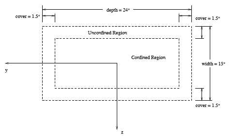
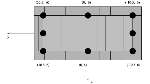
The dimension of the section are as shown in the figure. The section depth is 24 inches, the width 15 inches, and there is 1.5inch cover all around. Strong axis bending is about the z-axis. The section is separated into confined and unconfined concrete regions, for which separate discretizations will be generated, Reinforcing steel is placed around the boundary of th confined and unconfined regions. The fiber discretization is shown below:
The following are the commands that generate the section and perform the moment curvature analysis. The model and analysis commands are contained in the MomentCurvature procedure. These are contained in a seperate file which are "sourced"" by the main script.
# units: kip, in

# Remove existing model
wipe

# Create ModelBuilder (with two-dimensions and 3 DOF/node)
model BasicBuilder -ndm 2 -ndf 3

# Define materials for nonlinear columns
# ------------------------------------------
# CONCRETE                  tag   f'c        ec0   f'cu   ecu
# Core concrete (confined)
uniaxialMaterial Concrete01  1  -6.0  -0.004   -5.0     -0.014

# Cover concrete (unconfined)
uniaxialMaterial Concrete01  2  -5.0   -0.002   0.0     -0.006

# STEEL
# Reinforcing steel
set fy 60.0;      # Yield stress
set E 30000.0;    # Young's modulus
#                        tag  fy E0    b
uniaxialMaterial Steel01  3  $fy $E 0.01

# ------------------------------------------

# set some paramaters
set colWidth 15
set colDepth 24

set cover  1.5
set As    0.60;     # area of no. 7 bars

# some variables derived from the parameters
set y1 [expr $colDepth/2.0]
set z1 [expr $colWidth/2.0]
# Define cross-section for nonlinear columns

section Fiber 1 {

    # Create the concrete core fibers
    patch rect 1 10 1 [expr $cover-$y1] [expr $cover-$z1] [expr $y1-$cover] [expr $z1-$cover]

    # Create the concrete cover fibers (top, bottom, left, right)
    patch rect 2 10 1  [expr -$y1] [expr $z1-$cover] $y1 $z1
    patch rect 2 10 1  [expr -$y1] [expr -$z1] $y1 [expr $cover-$z1]
    patch rect 2  2 1  [expr -$y1] [expr $cover-$z1] [expr $cover-$y1] [expr $z1-$cover]
    patch rect 2  2 1  [expr $y1-$cover] [expr $cover-$z1] $y1 [expr $z1-$cover]

    # Create the reinforcing fibers (left, middle, right)
    layer straight 3 3 $As [expr $y1-$cover] [expr $z1-$cover] [expr $y1-$cover] [expr $cover-$z1]
    layer straight 3 2 $As 0.0 [expr $z1-$cover] 0.0 [expr $cover-$z1]
    layer straight 3 3 $As [expr $cover-$y1] [expr $z1-$cover] [expr $cover-$y1] [expr $cover-$z1]

}

# Estimate yield curvature
# (Assuming no axial load and only top and bottom steel)
set d [expr $colDepth-$cover]	;# d -- from cover to rebar
set epsy [expr $fy/$E]	;# steel yield strain
set Ky [expr $epsy/(0.7*$d)]

# Print estimate to standard output
puts "Estimated yield curvature: $Ky"

# Set axial load
set P -180

set mu 15;		# Target ductility for analysis
set numIncr 100;	# Number of analysis increments

# Call the section analysis procedure
MomentCurvature 1 $P [expr $Ky*$mu] $numIncr
Moment Curvature Procedure
The Tcl procedure to perform the moment-curvature analysis follows. The procedure takes as input the tag of the section to be analyzed, the axial load, P, to be applied, the max curvature to be evaluated and the number of iterations to achieve this max curavature.
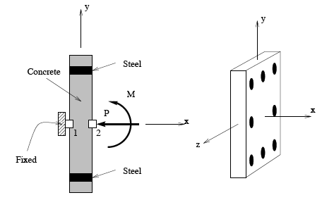
The procedure first creates the model which consists of two nodes, boundary conditions, and a ZeroLengthSection element. A depiction of the geometry is as shown in the top most figure above. The image on the left shows an edge view of the element, with local z-axis coming out of the page. Node 1 is completely restrained, with the applied loads acting at Node 2. An axial load, P, is applied to the section during the moment curvature analysis.
After the model has been created, the analysis is performed. A single load step is first performed for the axial load, then the integrator is changed to DisplacementControl to impose nodal displacements, which map directly to section deformations. A reference moment of 1.0 is defined in a Linear time series. For this reference moment, the DisplacementControl integrator will determine the load factor needed to apply the imposed displacement. A node recorder is defined to track the momentcurvature results. The load factor is the moment, and the nodal rotation is in fact the curvature of the element with zero thickness.
proc MomentCurvature {secTag axialLoad maxK {numIncr 100} } {
	# Define two nodes at (0,0)
	node 1 0.0 0.0
	node 2 0.0 0.0

	# Fix all degrees of freedom except axial and bending
	fix 1 1 1 1
	fix 2 0 1 0

	# Define element
	#                         tag ndI ndJ  secTag
	element zeroLengthSection  1   1   2  $secTag

	# Create recorder
	recorder Node -file section$secTag.out -time -node 2 -dof 3 disp

	# Define constant axial load
	pattern Plain 1 "Constant" {
		load 2 $axialLoad 0.0 0.0
	}

	# Define analysis parameters
	integrator LoadControl 0.0
	system SparseGeneral -piv;	# Overkill, but may need the pivoting!
	test NormUnbalance 1.0e-9 10
	numberer Plain
	constraints Plain
	algorithm Newton
	analysis Static

	# Do one analysis for constant axial load
	analyze 1

	# Define reference moment
	pattern Plain 2 "Linear" {
		load 2 0.0 0.0 1.0
	}

	# Compute curvature increment
	set dK [expr $maxK/$numIncr]

	# Use displacement control at node 2 for section analysis
	integrator DisplacementControl 2 3 $dK

	# Do the section analysis
	analyze $numIncr
}
Results
When you run this script, you should see the following printed to the screen:
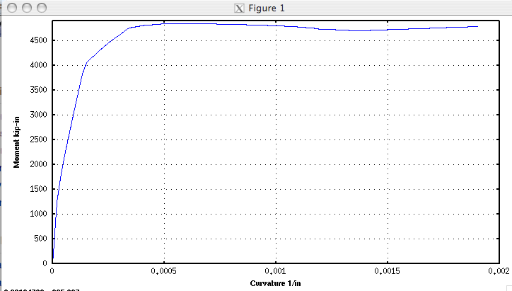
In addition, your directory should contain the following a file section1.out. A plot of this file using the following matlab commands
load section1.out
plot(section1(:,2),sections1(:,1)
xlabel("Curvature 1/in")
ylabel("Moment kip-in")
will produce the following: