Calibration of Maxwell Material: Difference between revisions
No edit summary |
No edit summary |
||
| (16 intermediate revisions by the same user not shown) | |||
| Line 1: | Line 1: | ||
Example posted by: <span style="color:blue"> Dr. Dimitrios G. Lignos | Example posted by: <span style="color:blue"> Dr. Dimitrios G. Lignos (McGill University)</span> | ||
---- | ---- | ||
| Line 6: | Line 6: | ||
The files needed to analyze this structure in OpenSees are included here: | The files needed to analyze this structure in OpenSees are included here: | ||
* The main file: [[Maxwell_Calibrator.tcl|Maxwell_Calibrator.tcl]] | * The main file: [[File:Maxwell_Calibrator.tcl|Maxwell_Calibrator.tcl]] | ||
Supporting procedure files | Supporting procedure files | ||
* [[SquareSsection.tcl|SquareSsection.tcl]] – displays a square fiber section | * [[File:SquareSsection.tcl|SquareSsection.tcl]] – displays a square fiber section | ||
* [[ | * [[File:ViscousD.tcl|ViscousD.tcl]] – contains the displacement loading history of the damper in units of mm | ||
All files are available in a compressed format here: [[Media:Calibration_Maxwell_example.zip|Calibration_Maxwell_example.zip]] | All files are available in a compressed format here: [[Media:Calibration_Maxwell_example.zip|Calibration_Maxwell_example.zip]] | ||
| Line 17: | Line 17: | ||
== Model Description == | == Model Description == | ||
[[File: | [[File:Maxwell-Fig1.png|300px|thumb|left|Figure 1. Schematic representation of a viscous damper.]] | ||
The viscous damper is modeled with the [[ | The viscous damper is modeled with the [[Force-Based Beam-Column Element|Force-Based Beam-Column element]]. This element follow a [[Maxwell Material| Maxwell]] hysteretic response. An idealized schematic of the model is presented in Figure 1. | ||
The units of the model are mm, N, and seconds. | The units of the model are mm, N, and seconds. | ||
=== Basic Geometry === | === Basic Geometry === | ||
| Line 28: | Line 29: | ||
=== Damper Section === | === Damper Section === | ||
A square section is used to define the area A of the damper (A<sub>damper</sub> = | A square section is used to define the area A of the damper (A<sub>damper</sub> = 12000.0mm<sup>2</sup>). | ||
=== Damper Links === | === Damper Links === | ||
[[ | [[Force-Based Beam-Column Element|Force-Based Beam-Column elements]] are used to link the two nodes that define the geometry of the viscous damper with n=5 sections of integration and the damper section defined previously. | ||
=== Constraints === | === Constraints === | ||
| Line 47: | Line 48: | ||
=== Recorders === | === Recorders === | ||
The [[Recorder Command|recorders]] used in this example include: | The [[Recorder Command|recorders]] used in this example include: | ||
* The [[ | * The [[Recorder Command|localForce recorder]] to track the axial force of the viscous damper | ||
* The [[ | * The [[Recorder Command|stressStrain recorder]] to track the stress and strain history of the viscous damper in section 3. | ||
=== Analysis === | === Analysis === | ||
| Line 55: | Line 56: | ||
== Results == | == Results == | ||
=== Comparison of OpenSees | === Comparison of OpenSees Model with MATLAB based Maxwell model === | ||
[[File: | [[File:MaxK1.png|300px|thumb|Right|Figure 2. Viscous Damper Response and Comparison With MATLAB based Script]] | ||
The force - displacement relationship from the maxwell damper are shown in Figure 2. In order to obtain the displacement of the damper we multiply the strain in section 3 of the damper times the length L=5000mm. A comparison of the response with a MATLAB based script is also shown in the same figure. Results are identical. | |||
Latest revision as of 00:38, 28 February 2011
Example posted by: Dr. Dimitrios G. Lignos (McGill University)
This example demonstrates how to conduct a calibration of a viscous damper using the maxwell model.
The files needed to analyze this structure in OpenSees are included here:
- The main file: File:Maxwell Calibrator.tcl
Supporting procedure files
- File:SquareSsection.tcl – displays a square fiber section
- File:ViscousD.tcl – contains the displacement loading history of the damper in units of mm
All files are available in a compressed format here: Calibration_Maxwell_example.zip
The rest of this example describes the model and shows the analysis results.
Model Description

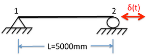
The viscous damper is modeled with the Force-Based Beam-Column element. This element follow a Maxwell hysteretic response. An idealized schematic of the model is presented in Figure 1.
The units of the model are mm, N, and seconds.
Basic Geometry
The basic geometry of the viscous damper is defined by input variables for the length L=5000mm, and area A = 12000mm2. Two nodes are used for the geometry of the damper.
Damper Section
A square section is used to define the area A of the damper (Adamper = 12000.0mm2).
Damper Links
Force-Based Beam-Column elements are used to link the two nodes that define the geometry of the viscous damper with n=5 sections of integration and the damper section defined previously.
Constraints
Node 1 is pinned. A roller is assigned to node 2
Maxwell Material
To model the viscous damper the Maxwell is used. The input parameters that are selected for the damper example are as follows: Axial Stiffness K = 500000.0 N/mm, Viscous Coefficient C=100000.0 N(s/mm)0.30 and exponent a=0.30.
Loading
The viscous damper is loaded with a displacement history that is called Damper.txt in the axial loading direction. A linear pattern is selected and the node of application is Node 2.
Recorders
The recorders used in this example include:
- The localForce recorder to track the axial force of the viscous damper
- The stressStrain recorder to track the stress and strain history of the viscous damper in section 3.
Analysis
In order to calibrate the viscous damper a multiple support excitation option is selected with application of displacement as the imposed motion. This is necessary since an integration step dt should be specified for integration of strain histories for each time step.
Results
Comparison of OpenSees Model with MATLAB based Maxwell model

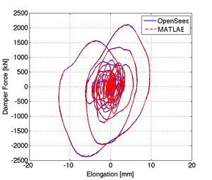
The force - displacement relationship from the maxwell damper are shown in Figure 2. In order to obtain the displacement of the damper we multiply the strain in section 3 of the damper times the length L=5000mm. A comparison of the response with a MATLAB based script is also shown in the same figure. Results are identical.